Skip to content

Watch & Learn
Practice
- Check My Competency
- Check My Exam Readiness
Ask a Trainer
Login

Excel Competency

Time limit: 0

Assessment Summary

0 of 40 Questions completed

Questions:

Information

You have already completed the assessment before. Hence you can not start it again.

Assessment is loading…

You must sign in or sign up to start the assessment.

You must first complete the following:

Results

Assessment complete. Results are being recorded.

Results

0 of 40 Questions answered correctly

Your time:

Time has elapsed

You have reached 0 of 0 point(s), (0)

Earned Point(s): 0 of 0, (0)
0 Essay(s) Pending (Possible Point(s): 0)

Categories

Not categorized 0%

You’re a Basic Excel user!

Back To Practice
You’re an Intermediate Excel user!

Back To Practice
You’re an Advanced Excel user!

Back To Practice

1
2
3
4
5
6
7
8
9
10
11
12
13
14
15
16
17
18
19
20
21
22
23
24
25
26
27
28
29
30
31
32
33
34
35
36
37
38
39
40

Current
Review
Answered
Correct
Incorrect

Question 1 of 40

1. Question
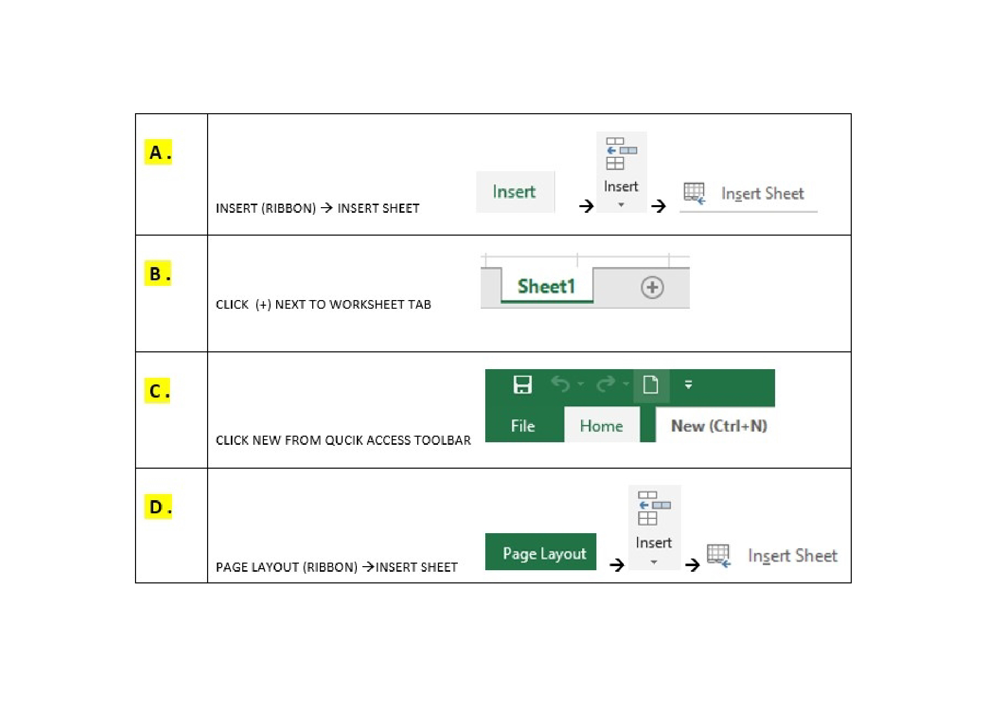
Q1. You need to add a new worksheet to your current file. How do insert an additional worksheet?
- A. INSERT (RIBBON) –> INSERT SHEET
- B. CLICK (+) NEXT TO WORKSHEET TAB
- C. CLICK NEW FROM QUCIK ACCESS TOOLBAR
- D. PAGE LAYOUT (RIBBON) –> INSERT SHEET
- E. I DON'T KNOW THE CORRECT ANSWER
Question 2 of 40

2. Question
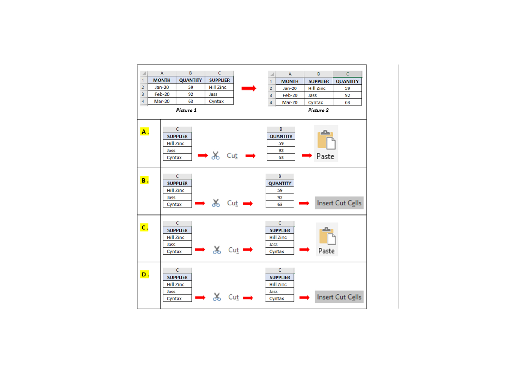
Q2. In Picture 1, the “SUPPLIER” column is located at column C. You would like to move the “SUPPLIER” column to column B as shown in Picture 2. How do you achieve this?
- A. SELECT COLUMN C –> CUT –> SELECT COLUMN B –> PASTE
- B. SELECT COLUMN C –> CUT –> RIGHT CLICK COLUMN B –> INSERT CUT CELLS
- C. SELECT COLUMN C –> CUT –> SELECT COLUMN C –> PASTE
- D. SELECT COLUMN C –> CUT –> RIGHT CLICK COLUMN C –> INSERT CUT CELLS
- E. I DON'T KNOW THE CORRECT ANSWER
Question 3 of 40

3. Question
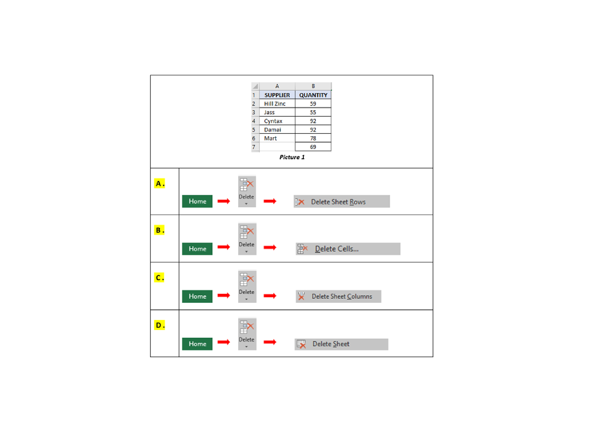
Q3. You have entered the value 92, twice in the “QUANTITY” column, as Picture 1. How to do remove the extra value?
- A. HOME (RIBBON) –> DELETE –> DELETE SHEET ROWS
- B. HOME (RIBBON) –> DELETE –> DELETE CELLS
- C. HOME (RIBBON) –> DELETE –> DELETE SHEET COLUMNS
- D. HOME (RIBBON) –> DELETE –> DELETE SHEET
- E. I DON'T KNOW THE CORRECT ANSWER
Question 4 of 40

4. Question
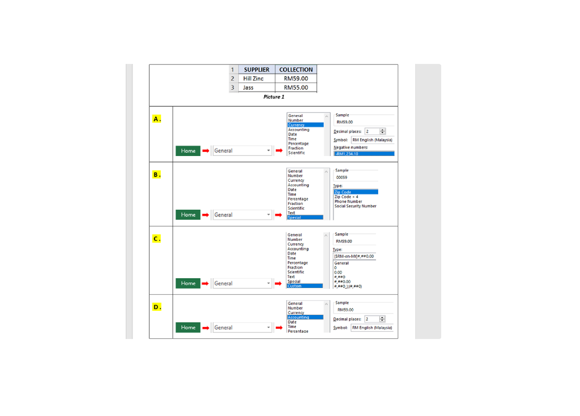
Q4. How do you apply the “RM” formatting to the values in column B as Picture 1?
- A. HOME (RIBBON) –> GENERAL –> CURRENCY (CATEGORY) –> CHOOSE SYMBOL AS RM
- B. HOME (RIBBON) –> GENERAL –> SPECIAL (CATEGORY) –> CHOOSE TYPE AS ZIP CODE
- C. HOME (RIBBON) –> GENERAL –> CUSTOM (CATEGORY) –> TYPE AS RM
- D. HOME (RIBBON) –> GENERAL –> ACCOUNTING (CATEGORY) –> CHOOSE SYMBOL AS RM
- E. I DON'T KNOW THE CORRECT ANSWER
Question 5 of 40

5. Question
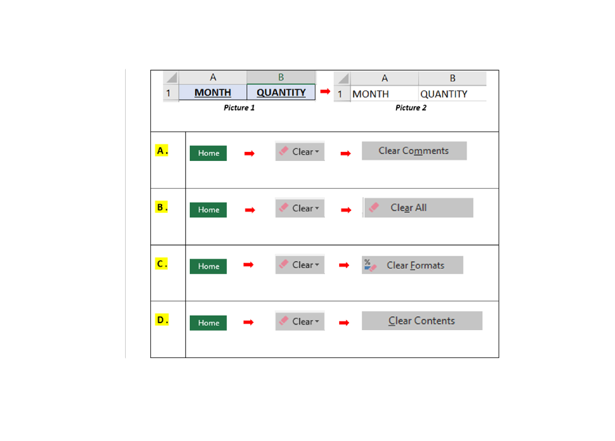
Q5. The range A1:B1 have the border, fill color and font styles as Picture 1. You want the result as Picture 2. Which of the following options would be able to accomplish this?
- A. HOME –> CLEAR –> CLEAR COMMENTS
- B. HOME –> CLEAR –> CLEAR ALL
- C. HOME –> CLEAR –> CLEAR FORMATS
- D. HOME –> CLEAR –> CLEAR CONTENS
- E. I DON'T KNOW THE CORRECT ANSWER
Question 6 of 40

6. Question
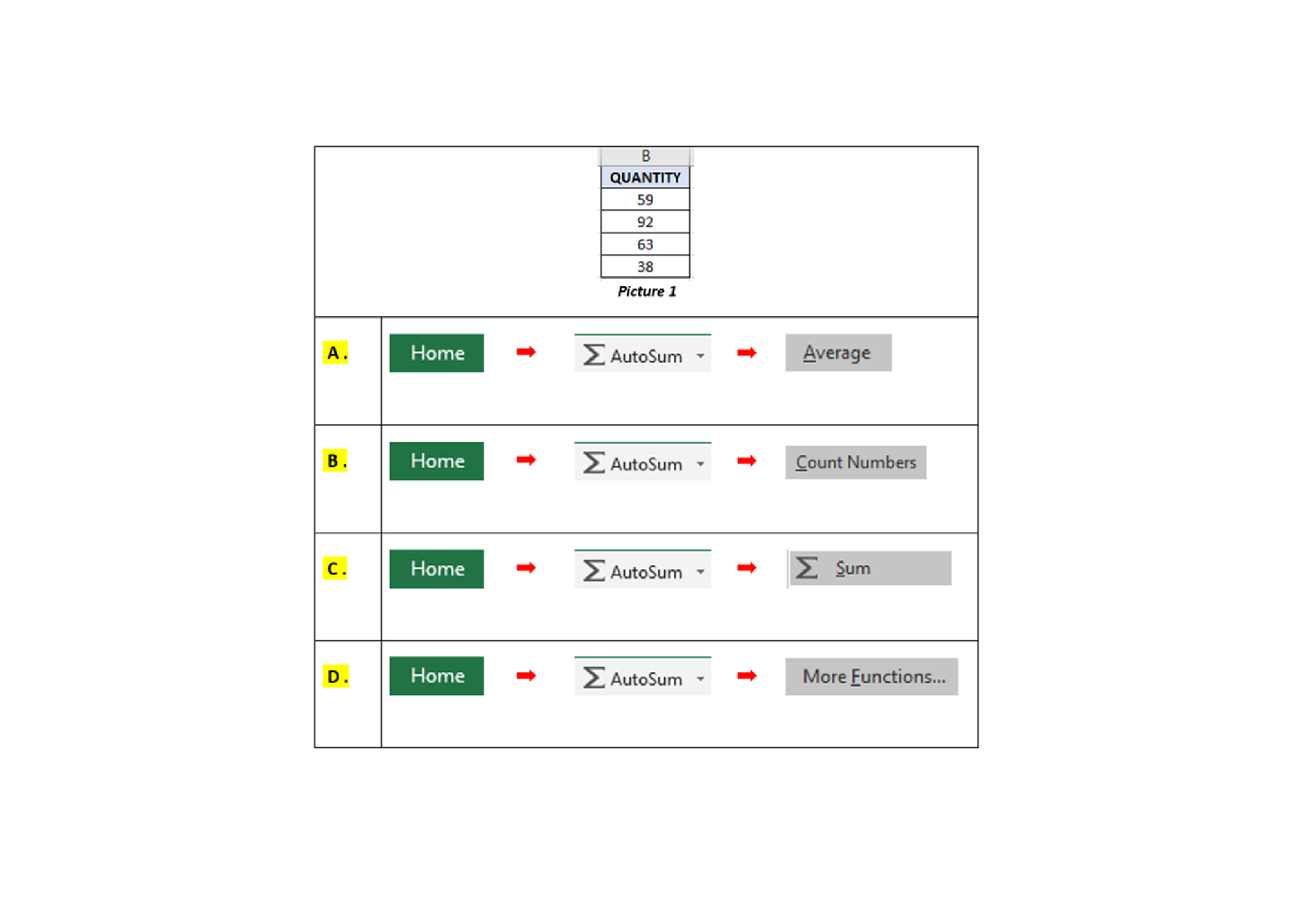
Q6. Which of the following options, will allow you to total up the values in the “QUANTITY” column as per the Picture 1?
- A. HOME –> AUTOSUM –> AVERAGE
- B. HOME –> AUTOSUM –> COUNT NUMBERS
- C. HOME –> AUTOSUM –> SUM
- D. HOME –> AUTOSUM –> MORE FUNCTIONS
- E. I DON'T KNOW THE CORRECT ANSWER
Question 7 of 40

7. Question
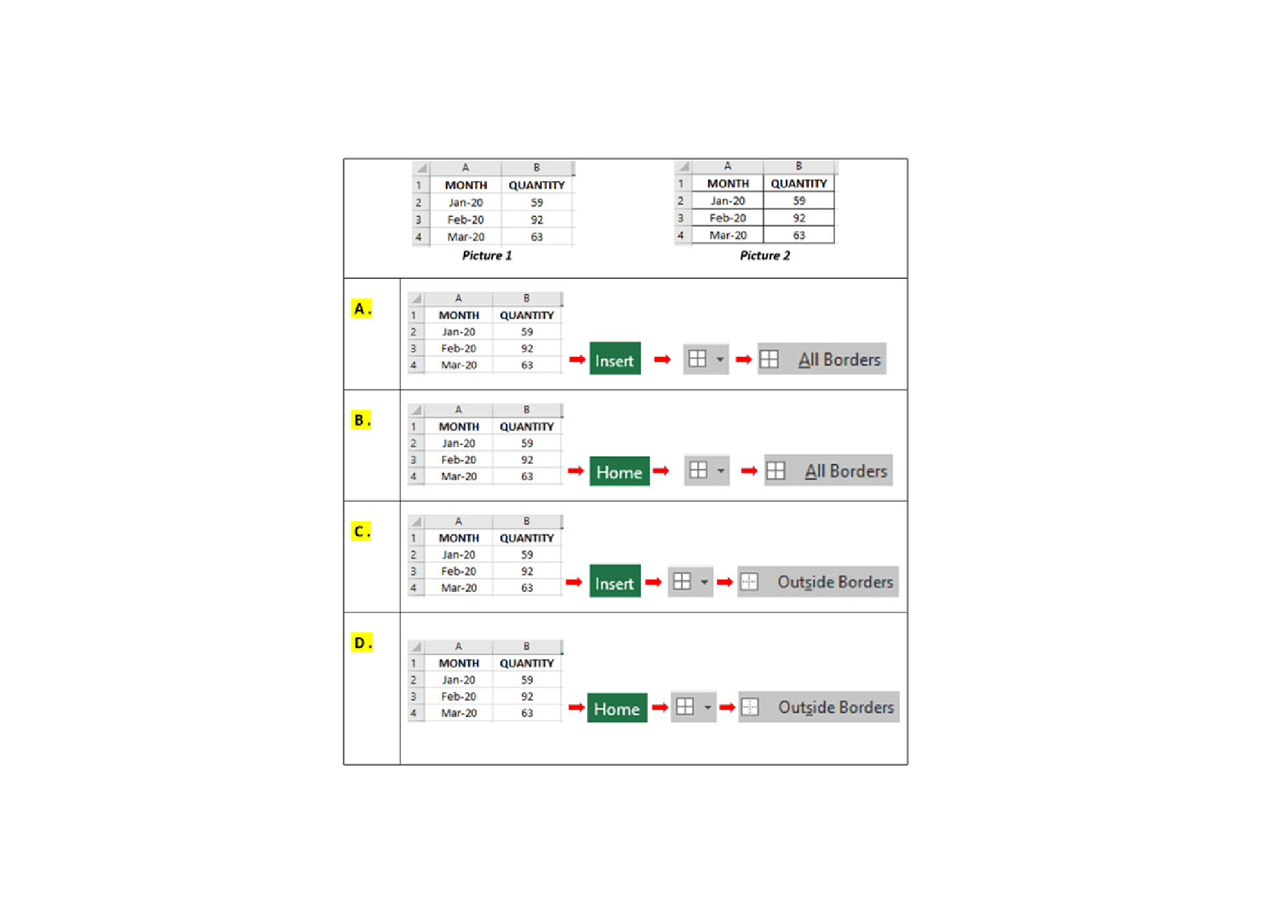
Q7. The range A1:B4 without border as Picture 1. How do you add borders as shown in the Picture 2?
- A. SELECT A1:B4 –> INSERT (RIBBON) –> ALL BORDERS
- B. SELECT A1:B4 –> HOME (RIBBON) –> ALL BORDERS
- C. SELECT A1:B4 –> INSERT (RIBBON) –> OUTSIDE BORDERS
- D. SELECT A1:B4 –> HOME (RIBBON) –> OUTSIDE BORDERS
- E. I DON'T KNOW THE CORRECT ANSWER
Question 8 of 40

8. Question
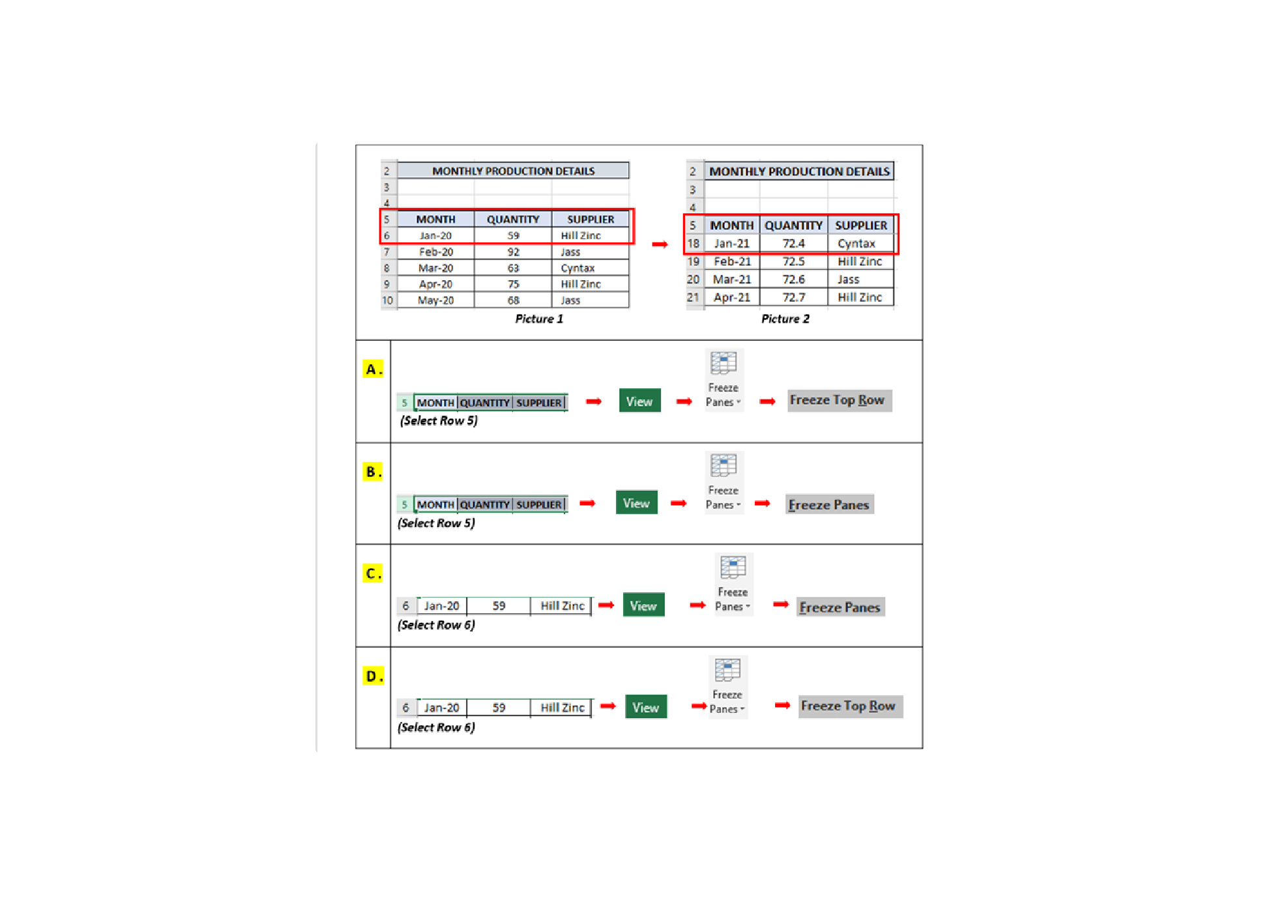
Q8. For the “Monthly Production Details” database, you would like to view the Jan-21 record at ROW 18. When scrolling down to search for your data, you want the header of “ROW 5” to be visible. Which of the following options will allow you to achieve this?
- A. SELECT ROW 5 –> VIEW (RIBBON) –> FREEZE PANES –> FREEZE TOP ROW
- B. SELECT ROW 5 –> VIEW (RIBBON) –> FREEZE PANES –> FREEZE PANES
- C. SELECT ROW 6 –> VIEW (RIBBON) –> FREEZE PANES –> FREEZE PANES
- D. SELECT ROW 6 –> VIEW (RIBBON) –> FREEZE PANES –> FREEZE TOP ROW
- E. I DON'T KNOW THE CORRECT ANSWER
Question 9 of 40

9. Question
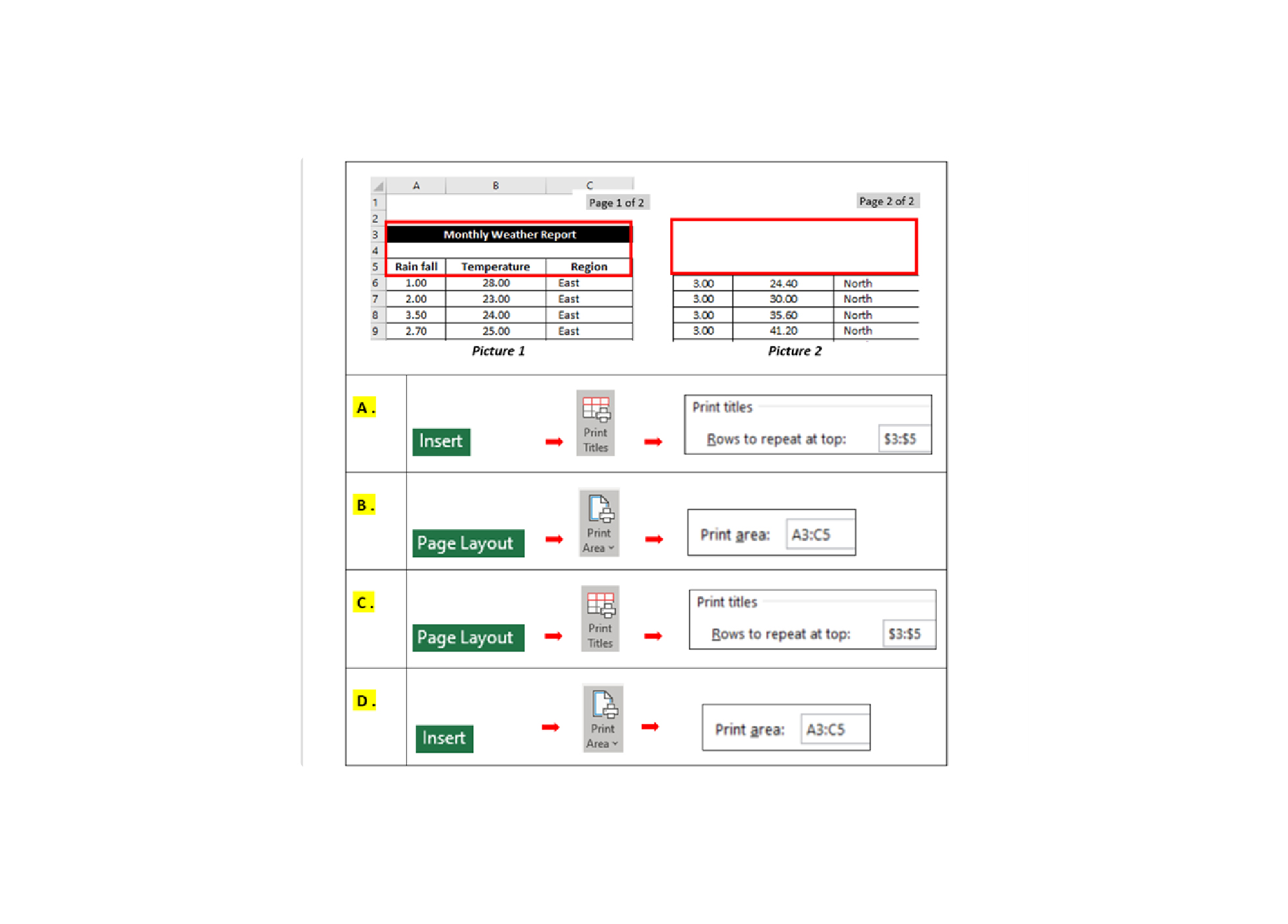
Q9. When printing your spreadsheet, your output is on 2-pages. How do you get the titles to repeat on the subsequent pages?
- A. INSERT (RIBBON –> PRINT TITLES –> ROWS TO REPEAT AT TOP $3:$5
- B. PAGE LAYOUT (RIBBON –> PRINT AREA –> A3:C5
- C. PAGE LAYOUT (RIBBON –> PRINT TITLES –> ROWS TO REPEAT AT TOP $3:$5
- D. INSERT (RIBBON –> PRINT AREA –> A3:C5
- E. I DON'T KNOW THE CORRECT ANSWER
Question 10 of 40

10. Question
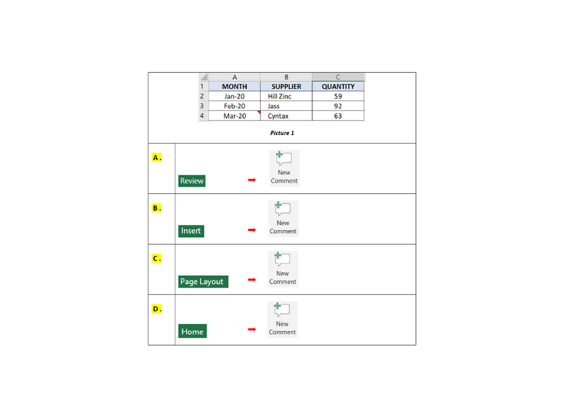
Q10. There is a “RED” triangle at the top right corner of the “Mar-20”. How do you create the “RED” triangle?
- A. REVIEW (RIBBON) –> NEW COMMENT
- B. INSERT (RIBBON) –> NEW COMMENT
- C. LAGE LAYOUT (RIBBON) –> NEW COMMENT
- D. HOME (RIBBON) –> NEW COMMENT
- E. I DON'T KNOW THE CORRECT ANSWER
Question 11 of 40

11. Question
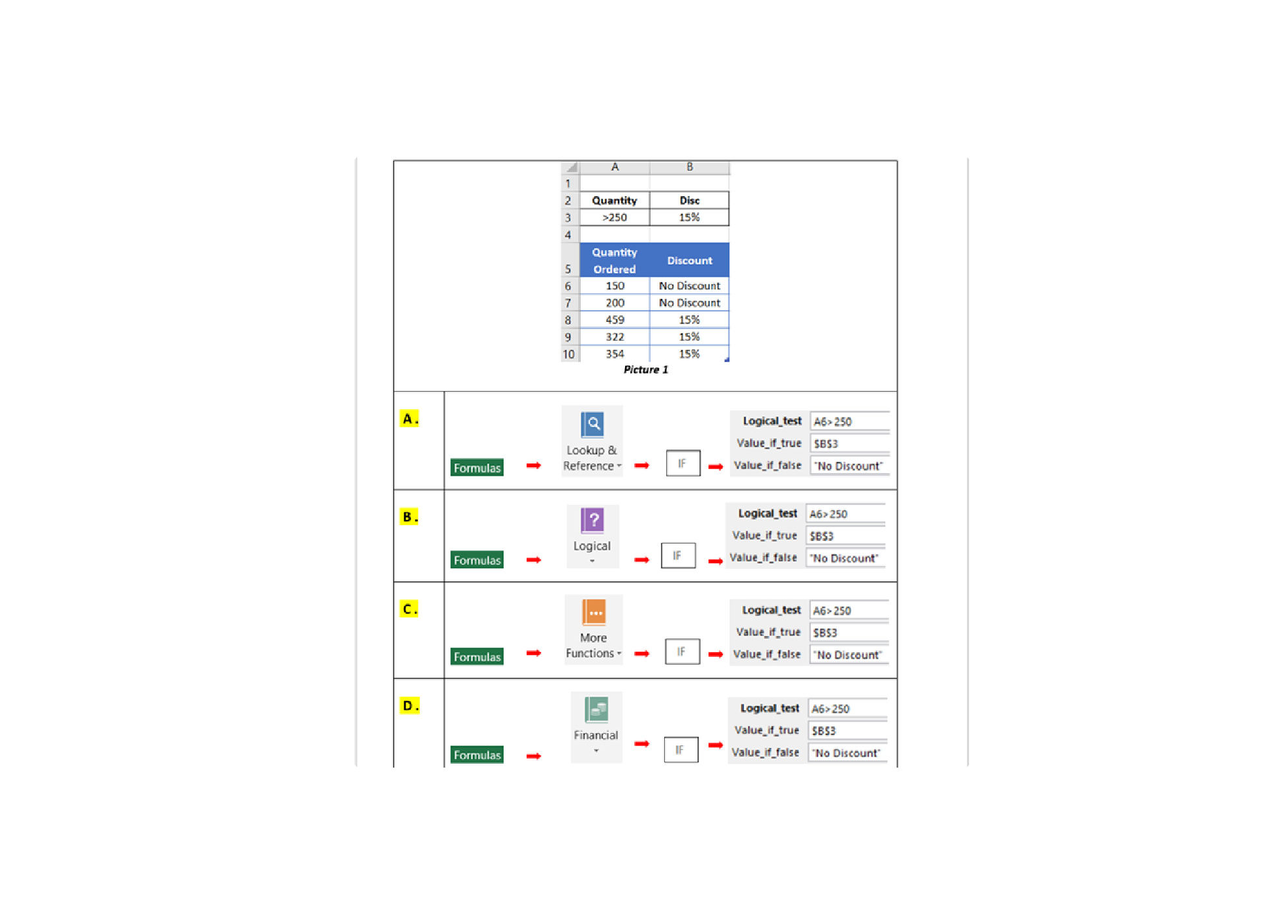
Q11. 15% discount is given, when the quantity ordered above 250 units. How do you create the “DISCOUNT” in B6:B10 as Picture 1?
- A. FORMULAS (RIBBON) –> LOOKUP & REFERENCE –> IF
- B. FORMULAS (RIBBON) –> LOGICAL –> IF
- C. FORMULAS (RIBBON) –> MORE FUNCTIONS –> IF
- D. FORMULAS (RIBBON) –> FINANCE –> IF
- E. I DON'T KNOW THE CORRECT ANSWER
Question 12 of 40

12. Question
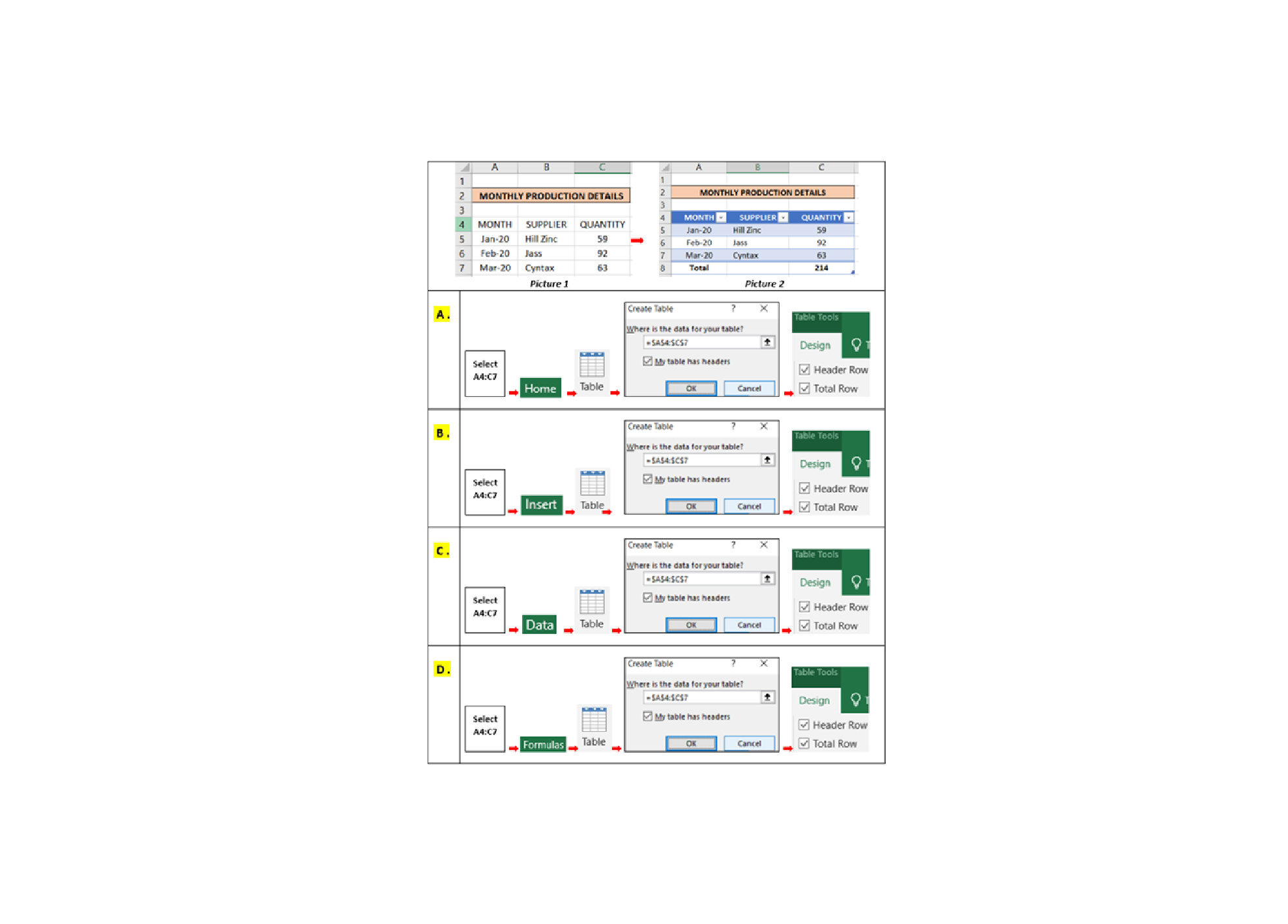
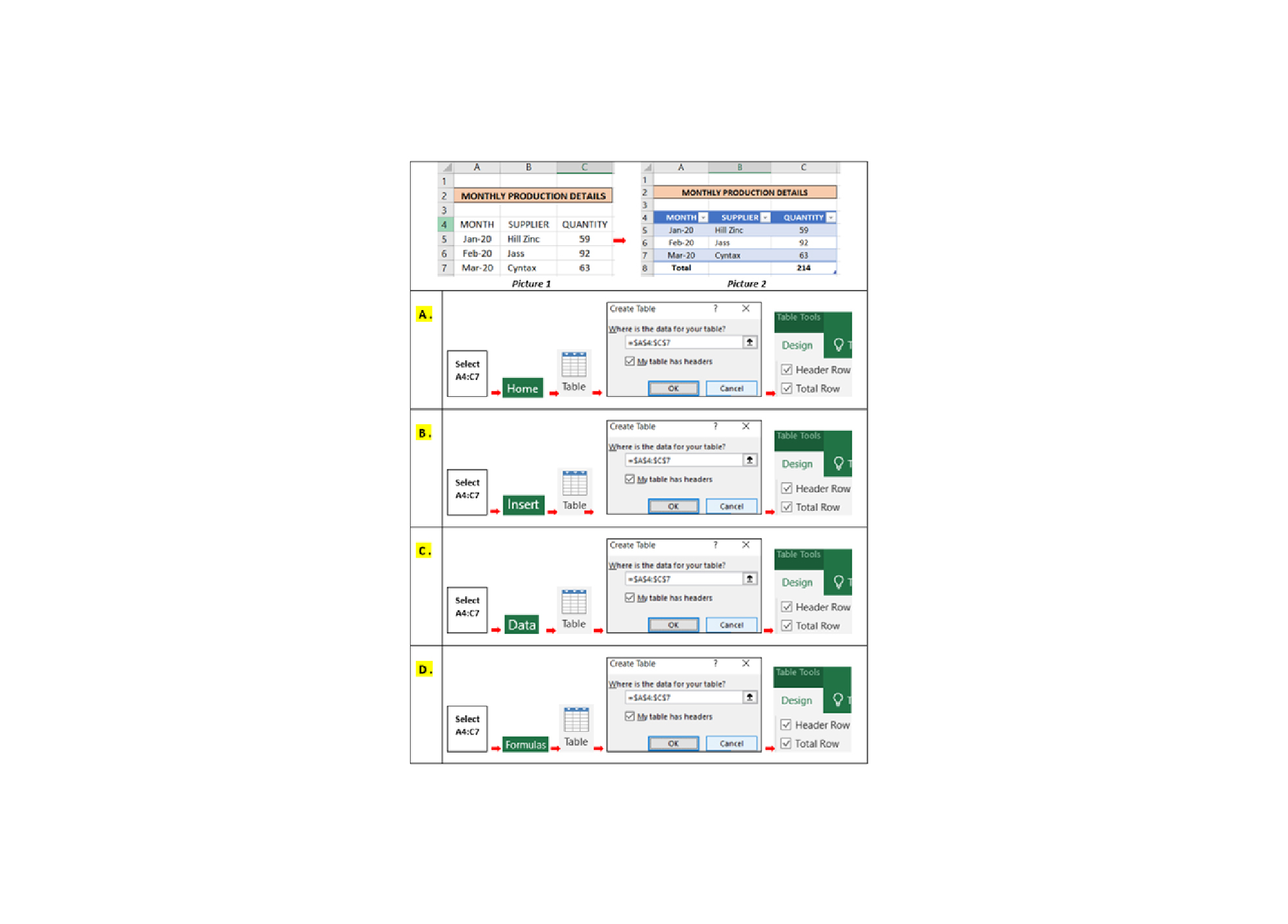
Q12. How to create a database as Picture 2 from data shown in Picture 1?
- A. SELECT A4:C7 –> HOME (RIBBON) –> TABLE –> CREATE TABLE (BOX) –> CLICK OK –> DESIGN (RIBBON) –> TOTAL ROW
- B. SELECT A4:C7 –> INSERT (RIBBON) –> TABLE –> CREATE TABLE (BOX) –> CLICK OK –> DESIGN (RIBBON) –> TOTAL ROW
- C. SELECT A4:C7 –> DATA (RIBBON) –> TABLE –> CREATE TABLE (BOX) –> CLICK OK –> DESIGN (RIBBON) –> TOTAL ROW
- D. SELECT A4:C7 –> FORMULAS (RIBBON) –> TABLE –> CREATE TABLE (BOX) –> CLICK OK –> DESIGN (RIBBON) –> TOTAL ROW
- E. I DON'T KNOW THE CORRECT ANSWER
Question 13 of 40

13. Question
Q13. How do you total all HILL ZINC’s Quantity that is above 80 units?
- A. FORMULAS (RIBBON) –> MORE FUNCTIONS –> DSUM
- B. FORMULAS (RIBBON) –> MATH & TRIG –> DSUM
- C. FORMULAS (RIBBON) –> DATABASE –> DSUM
- D. FORMULAS (RIBBON) –> LOOKUP & REFERENCE –> DSUM
- E. I DON'T KNOW THE CORRECT ANSWER
Question 14 of 40

14. Question
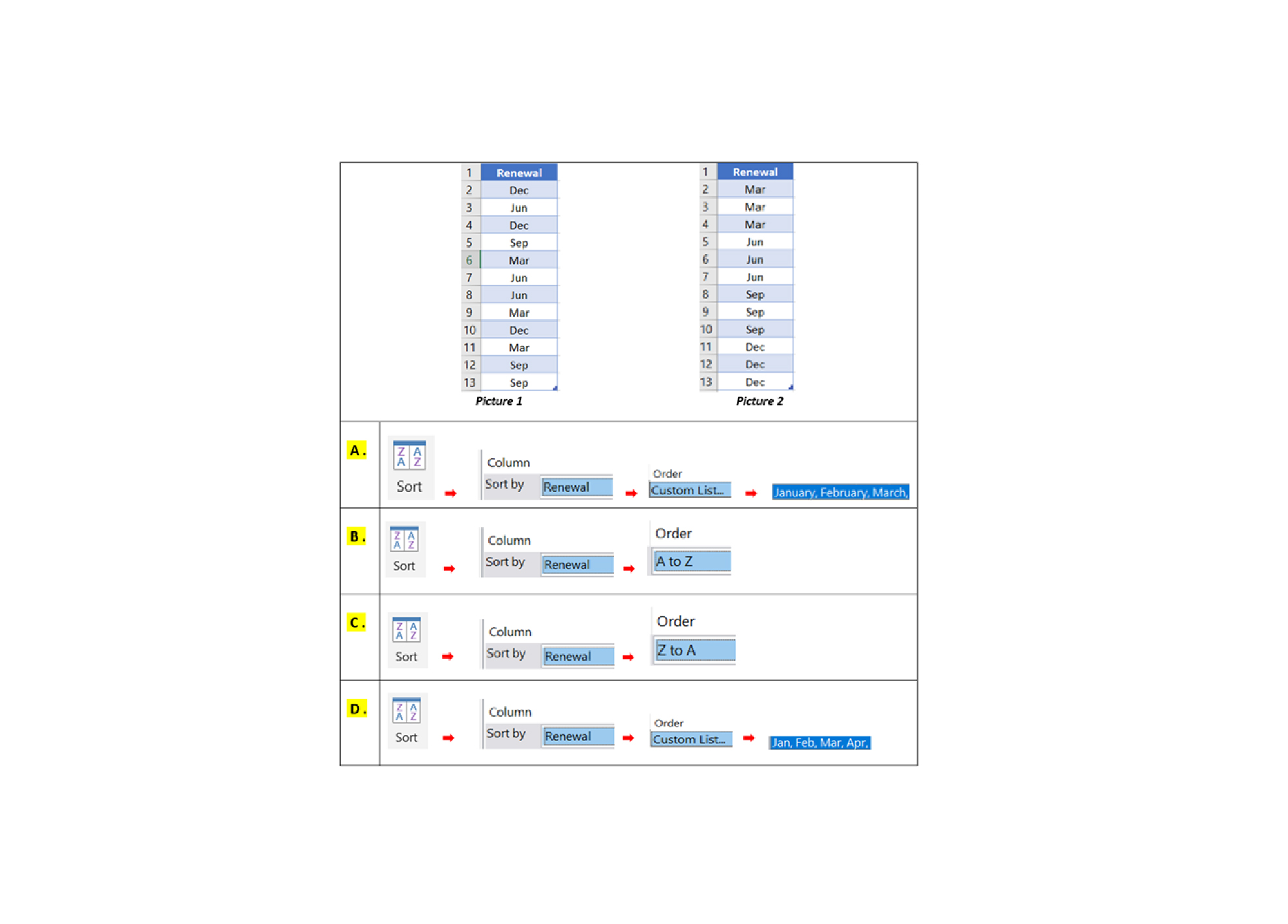
Q14. You would like to rearrange data in “RENEWAL” column by month as shown in Picture 2. Which methods will allow you to do this?
- A. SORT –> RENEWAL (COLUMN) –> CUSTOM LIST (ORDER) –> CHOOSE JANUANY,FEBRUARY,MARCH, …
- B. SORT –> RENEWAL (COLUMN) –> A TO Z (ORDER)
- C. SORT –> RENEWAL (COLUMN) –> Z TO A (ORDER)
- D. SORT –> RENEWAL (COLUMN) –> CUSTOM LIST (ORDER) –> CHOOSE JAN, FEB, MAR, …
- E. I DON'T KNOW THE CORRECT ANSWER
Question 15 of 40

15. Question
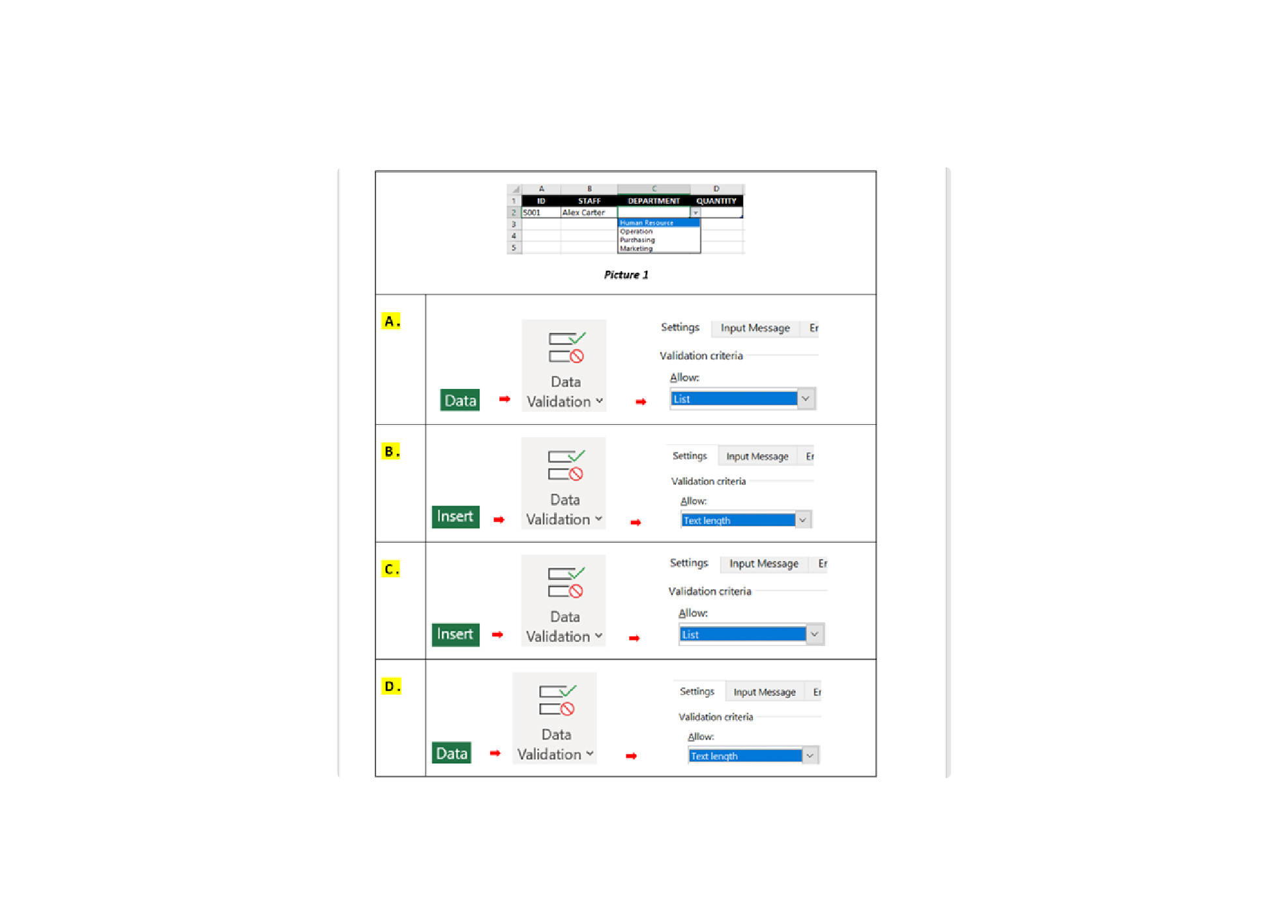
Q15. How do you create a drop-down list for the departments as shown in the Picture 1?
- A. DATA (RIBBON) –> DATA VALIDATION –> SETTINGS –> CHOOSE LIST (VALIDATION CRITERIA)
- B. INSERT (RIBBON) –> DATA VALIDATION –> SETTINGS –> CHOOSE TEXT LENGTH (VALIDATION CRITERIA)
- C. INSERT (RIBBON) –> DATA VALIDATION –> SETTINGS –> CHOOSE LIST (VALIDATION CRITERIA)
- D. DATA (RIBBON) –> DATA VALIDATION –> SETTINGS –> CHOOSE TEXT LENGTH (VALIDATION CRITERIA)
- E. I DON'T KNOW THE CORRECT ANSWER
Question 16 of 40

16. Question
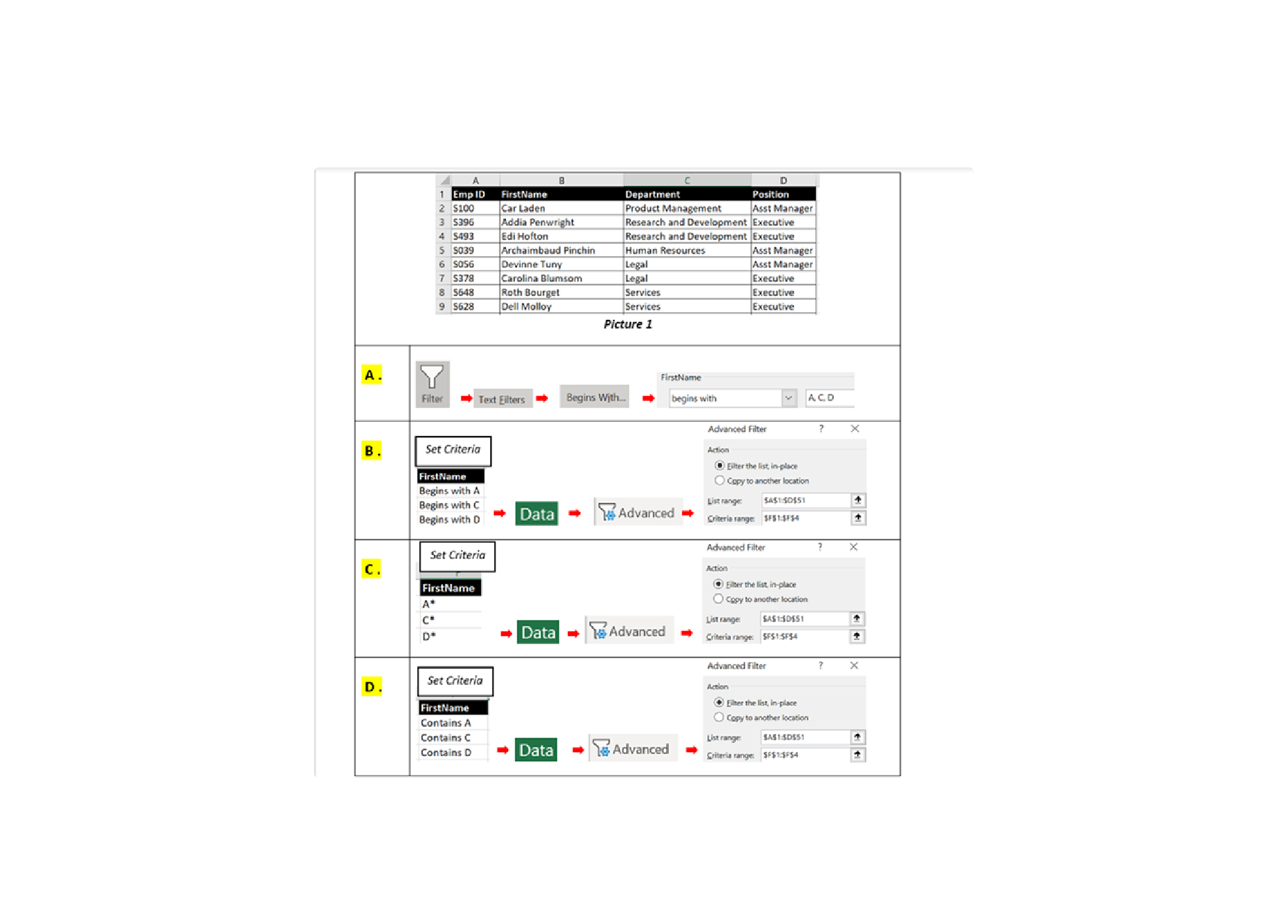
Q16. In the database below, you would like to filter “FIRSTNAME” that begins with “A”, “C” or “D”. Which of the following answers allows you achieve this?
- A. FILTER –> TEXT FILTERS –> BEGINS WITH –> key in A, B, C
- B. CRITERIA (BEGINS WITH A C D) –> DATA (RIBBON) –> ADVANCED –> LIST RANGE (A1:D51) and CRITERIA (F1:F4)
- C. CRITERIA (A* C* D*) –> DATA (RIBBON) –> ADVANCED –> LIST RANGE (A1:D51) and CRITERIA (F1:F4)
- D. CRITERIA (CONTAINS WITH A C D) –> DATA (RIBBON) –> ADVANCED –> LIST RANGE (A1:D51) and CRITERIA (F1:F4)
- E. I DON'T KNOW THE CORRECT ANSWER
Question 17 of 40

17. Question
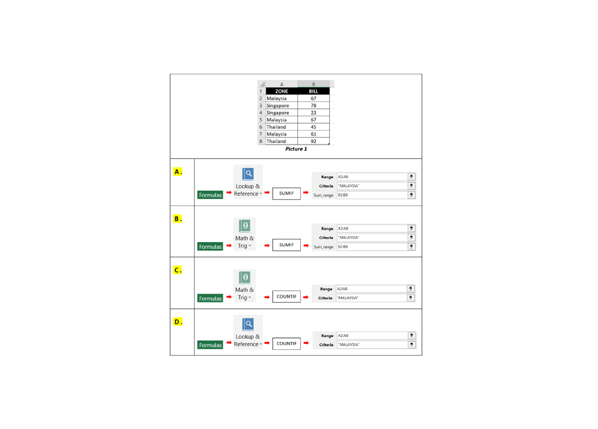
Q17. You would like to total all the “BILL” for “MALAYSIA” zone. Which of the following answers will allow you to do this?
- A. FORMULAS (RIBBON) –> LOOKUP & REFERENCE –> SUMIF
- B. FORMULAS (RIBBON) –> MATH & TRIG –> SUMIF
- C. FORMULAS (RIBBON) –> MATH & TRIG –> COUNTIF
- D. FORMULAS (RIBBON) –> LOOKUP & REFERENCE –> COUNTIFIF
- E. I DON'T KNOW THE CORRECT ANSWER
Question 18 of 40

18. Question
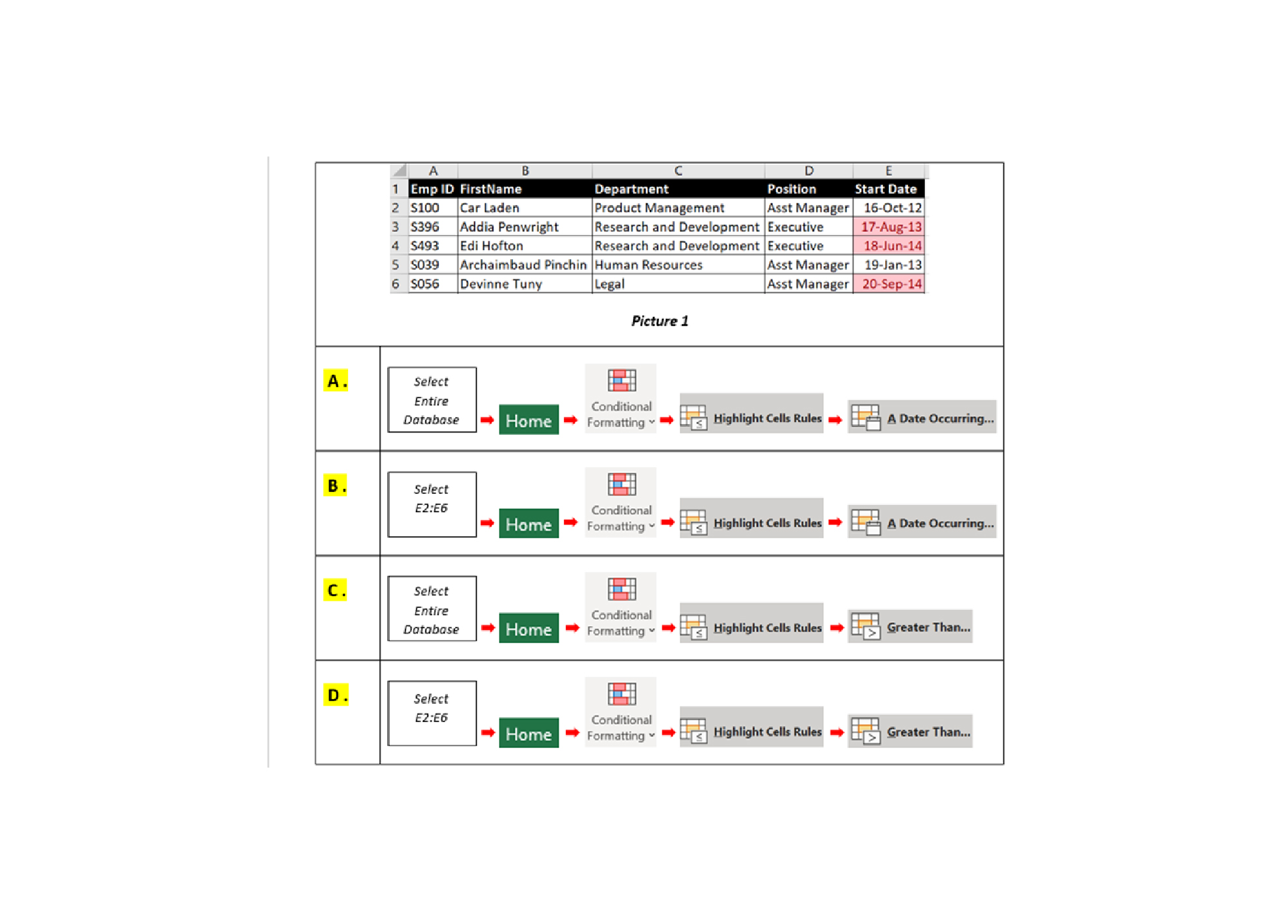
Q18. In the Employees’ database below, you would like to highlight all Start Date after 1st July, 2013. How do you do this?
- A. Select Entire Database > Home (Ribbon) > Conditional Formatting > Highlight Cell Rules –> A Date Occurring
- B. Select E2:E6 > Home (Ribbon) > Conditional Formatting > Highlight Cell Rules –> A Date Occurring
- C. Select Entire Database > Home (Ribbon) > Conditional Formatting > Highlight Cell Rules –> Greater Than
- D. Select E2:E6 > Home (Ribbon) > Conditional Formatting > Highlight Cell Rules –> Greater Than
- E. I DON'T KNOW THE CORRECT ANSWER
Question 19 of 40

19. Question
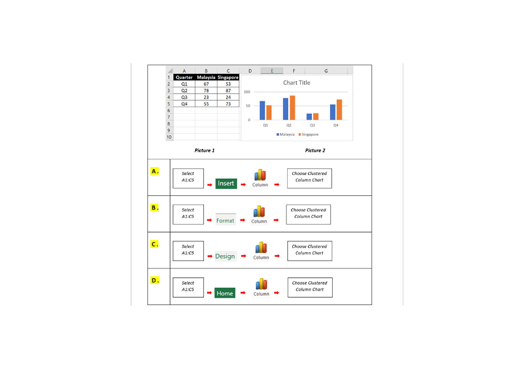
Q19. How do you create a chart, as shown in the picture below?
- A. SELECT A1:C5 –> INSERT (RIBBON) –> COLUMN –> Choose Clustered Column Chart
- B. SELECT A1:C5 –> FORMAT (RIBBON) –> COLUMN –> Choose Clustered Column Chart
- C. SELECT A1:C5 –> DESIGN (RIBBON) –> COLUMN –> Choose Clustered Column Chart
- D. SELECT A1:C5 –> HOME (RIBBON) –> COLUMN –> Choose Clustered Column Chart
- E. I DON'T KNOW THE CORRECT ANSWER
Question 20 of 40

20. Question
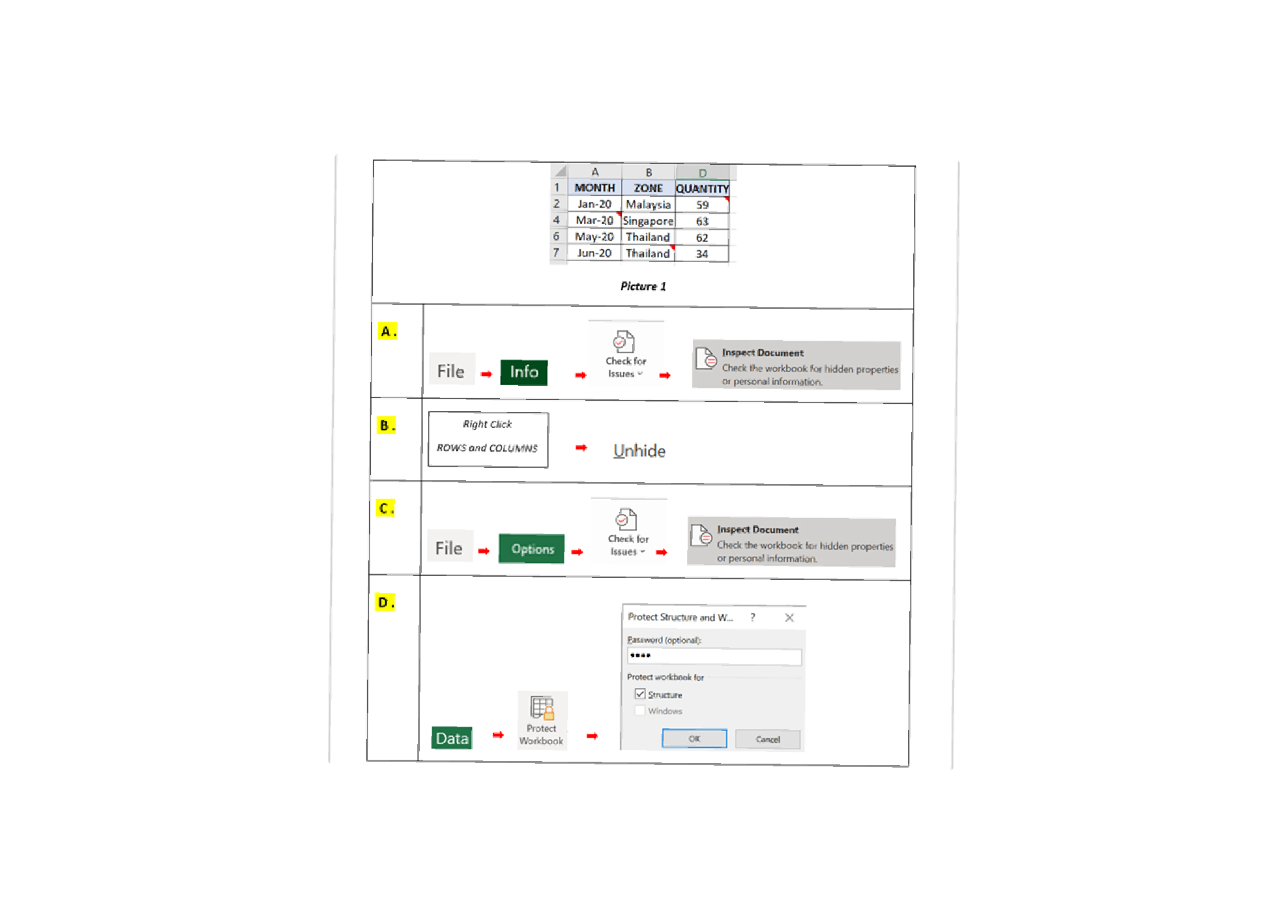
Q20. In the spreadsheet as Picture 1, there are “comments” and hidden rows and columns. You would like to remove all comments and unhide rows and columns from the spreadsheet. Which method will allow you to achieve this?
- A. FILE (TAB) –> INFO –> CHECK FOR ISSUES –> INSPECT DOCUMENT
- B. RIGHT CLICK ROWS and COLUMNS –> UNHIDE
- C. FILE (TAB) –> INFO –> CHECK FOR ISSUES –> INSPECT DOCUMENT
- D. DATA (RIBBON) –> PROTECT WORKBOOK –> ENTER PASSWORD –> CLICK OK
- E. I DON'T KNOW THE CORRECT ANSWER
Question 21 of 40

21. Question
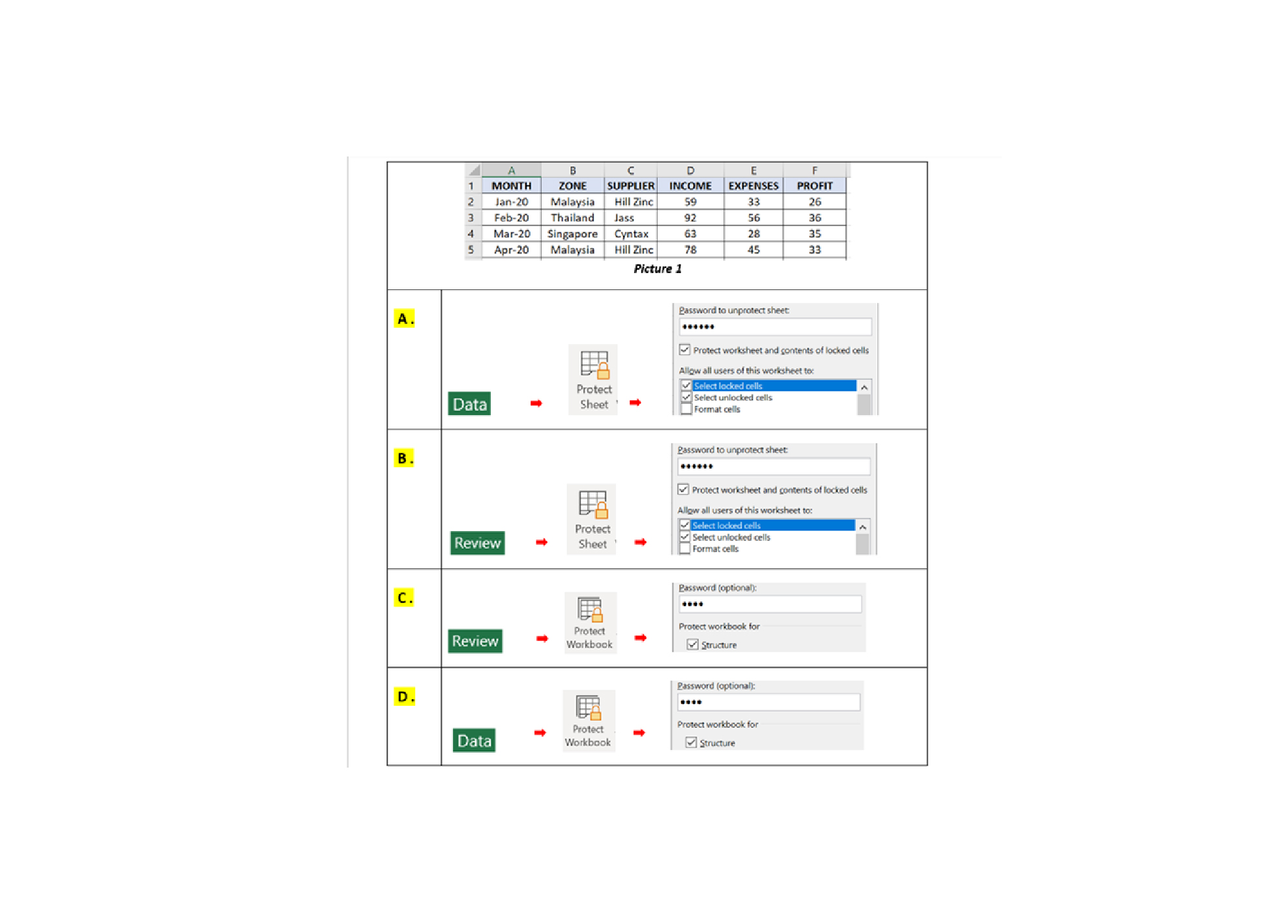
Q21. You have prepared an income and expenses report as Picture 1. This report needs to be sent to the marketing department, for their budget preparation. To ensure that they do not modify your report, you should apply PROTECTION settings. How do set protection in Excel?
- A. DATA (RIBBON) –> PROTECT SHEET –> ENTER PASSWORD
- B. REVIEW (RIBBON) –> PROTECT SHEET –> ENTER PASSWORD
- C. REVIEW (RIBBON) –> PROTECT WORKBOOK –> ENTER PASSWORD
- D. DATA (RIBBON) –> PROTECT WORKBOOK –> ENTER PASSWORD
- E. I DON'T KNOW THE CORRECT ANSWER
Question 22 of 40

22. Question
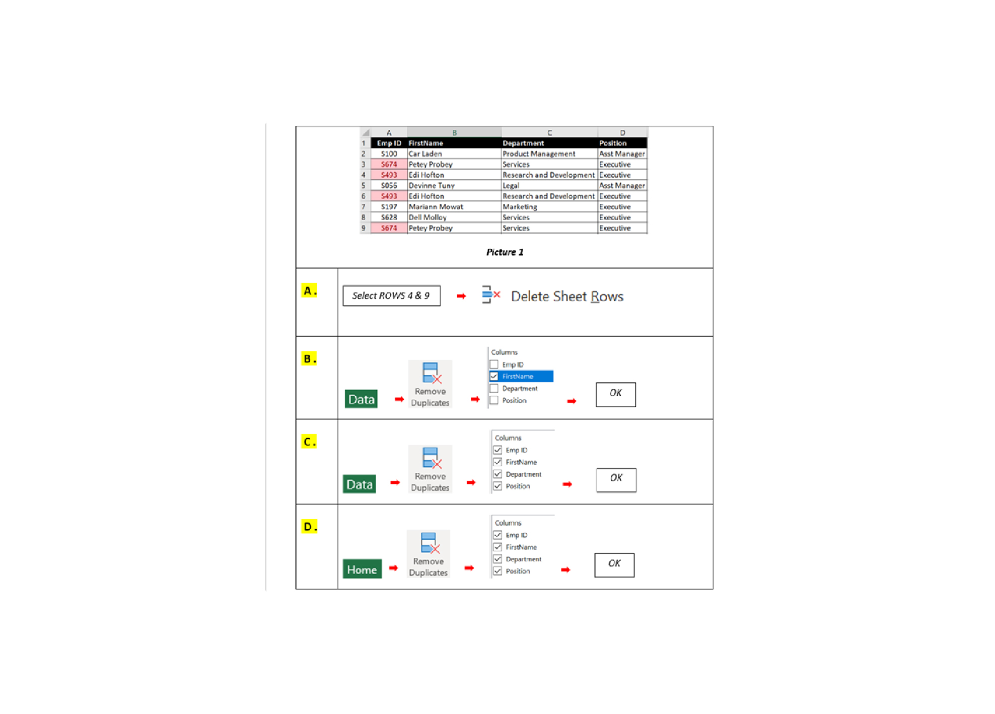
Q22. In database as Picture 1, you notice that there are 2-pairs of duplicate record. How do you remove the duplicate records?
- A. SELECT ROWS 4 & 9 –> DELETE SHEET ROWS
- B. DATA (RIBBON) –> REMOVE DUPLICATES –> SELECT FIRSTNAME (COLUMN) –> OK
- C. DATA (RIBBON) –> REMOVE DUPLICATES –> SELECT EMP ID, FIRSTNAME, DEPARTMENT, POSITION (COLUMN) –> OK
- D. HOME (RIBBON) –> REMOVE DUPLICATES –> SELECT EMP ID, FIRSTNAME, DEPARTMENT, POSITION (COLUMN) –> OK
- E. I DON'T KNOW THE CORRECT ANSWER
Question 23 of 40

23. Question
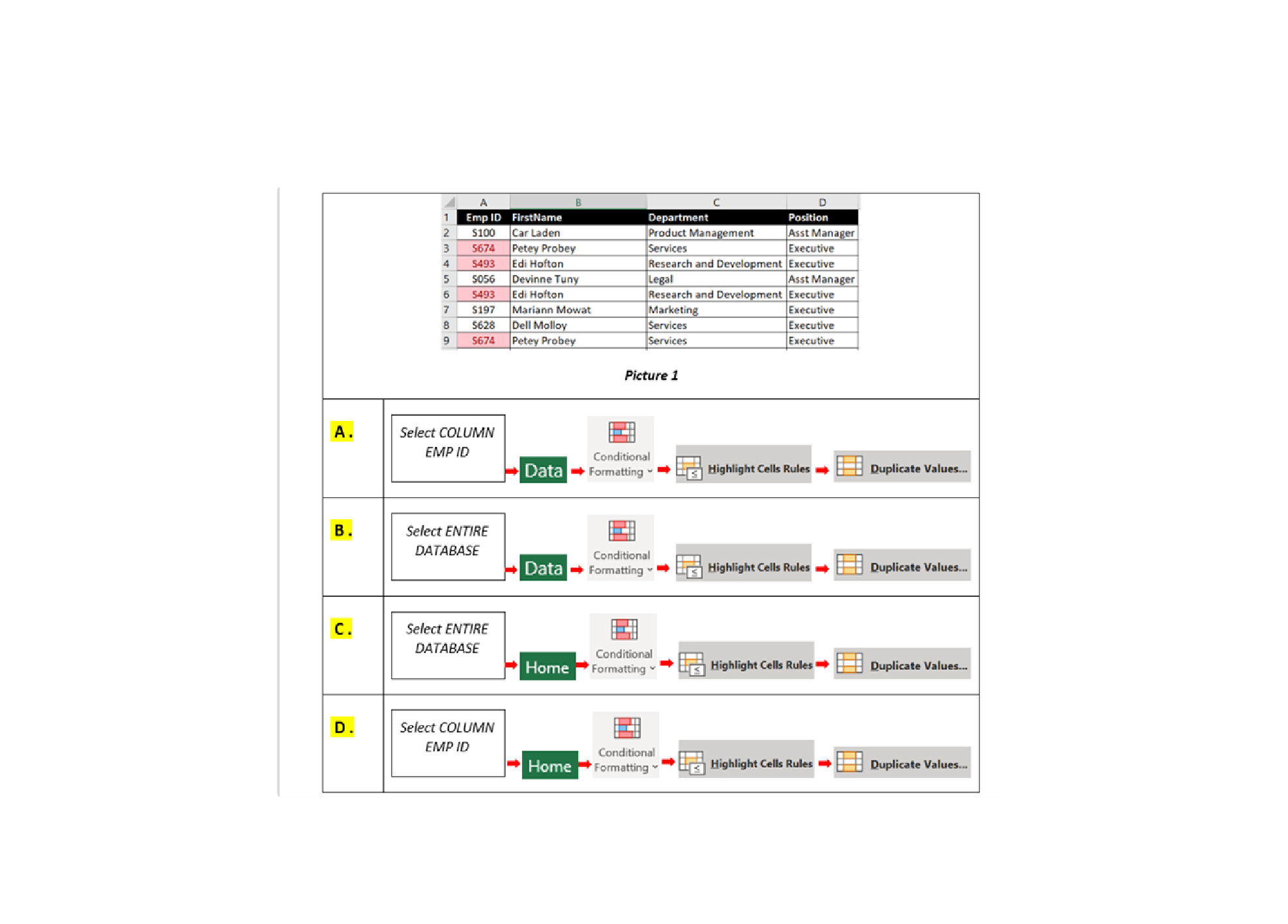
Q23. How do you identify duplicate data in the database below?
- A. SELECT EMP ID (COLUMN) –> DATA (RIBBON) –> CONDITIONAL FORMATTING –> HIGHLIGHT CELLS RULES — > DUPLICATE VALUE
- B. SELECT ENTIRE DATABASE –> DATA (RIBBON) –> CONDITIONAL FORMATTING –> HIGHLIGHT CELLS RULES — > DUPLICATE VALUE
- C. SELECT ENTIRE DATABASE –> HOME (RIBBON) –> CONDITIONAL FORMATTING –> HIGHLIGHT CELLS RULES – -> DUPLICATE VALUE
- D. SELECT EMP ID (COLUMN) –> HOME (RIBBON) –> CONDITIONAL FORMATTING –> HIGHLIGHT CELLS RULES –> DUPLICATE VALUE
- E. I DON'T KNOW THE CORRECT ANSWER
Question 24 of 40

24. Question
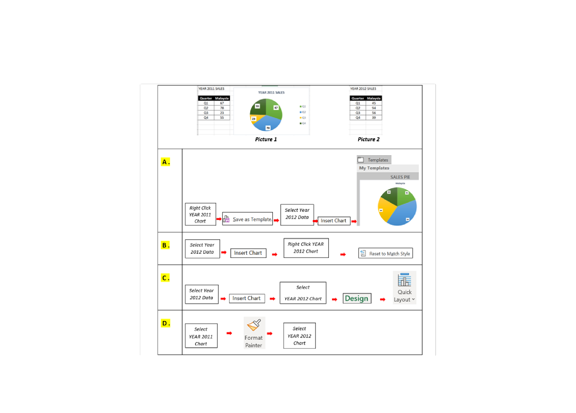
Q24. You have plotted a chart for Year 2011 Sales Performance and with custom style. For 2012 Sales Performance chart, you would like to apply the same style as 2011 style. How to do this?
- A. RIGHT CLICK “YEAR 2011 CHART” –> SAVE AS TEMPLATE –> SELECT “YEAR 2012 DATA” –> INSERT CHART –> TEMPLATE
- B. SELECT “YEAR 2012 DATA” –> INSERT CHART –> RIGHT CLICK “YEAR 2012 CHART” –> RESET TO MATCH STYLE
- C. SELECT “YEAR 2012 DATA” –> INSERT CHART –> SELECT “YEAR 2012 CHART” –> DESIGN (RIBBON) –> QUICK LAYOUT
- D. SELECT “YEAR 2011 CHART” –> FORMAT PAINTER –> SELECT “YEAR 2012 CHART”
- E. I DON'T KNOW THE CORRECT ANSWER
Question 25 of 40

25. Question
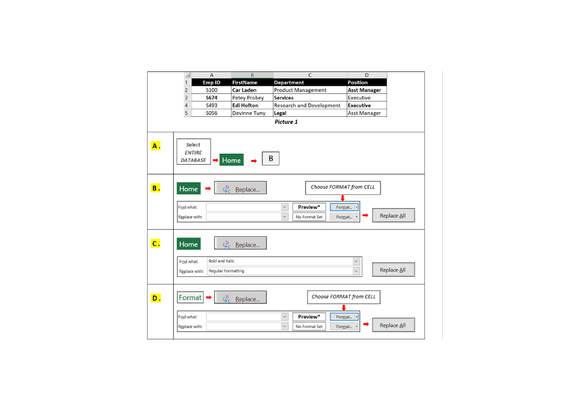
Q25. In your spreadsheet you have created some of cells with Font Style (Bold). But the cells across entire worksheet. You would like to remove all cells with Bold formatting to without Bold formatting. Which of the following method will allow you do this?
- A. SELECT ENTIRE DATABASE –> HOME (RIBBON) –> BOLD
- B. HOME (RIBBON) –> REPLACE –> FIND WHAT (CHOOSE FORMAT FROM CELL) –> REPLACE ALL
- C. HOME (RIBBON) –> REPLACE –> FIND WHAT (BOLD AND ITALIC) –> REPLACE WHAT (REGULAR FORMATTING) –> REPLACE ALL
- D. FORMAT (RIBBON) –> REPLACE –> FIND WHAT (CHOOSE FORMAT FROM CELL) –> REPLACE ALL
- E. I DON'T KNOW THE CORRECT ANSWER
Question 26 of 40

26. Question
Q26. How do you create the function that is boxed in RED in the picture below?
- A. DATA (RIBBON) –> FILTER –> SELECT ALL
- B. SELECT ROW 2:3, 5:6, 8:9 –> DATA –> GROUP
- C. DATA (RIBBON) –> AUTO OUTLINE
- D. DATA (RIBBON) –> SUBTOTAL –> AT EACH CHANGE IN (PRODUCT) –> USE FUNCTION (SUM) –> ADD SUBTOTAL JAN, FEB
- E. I DON'T KNOW THE CORRECT ANSWER
Question 27 of 40

27. Question
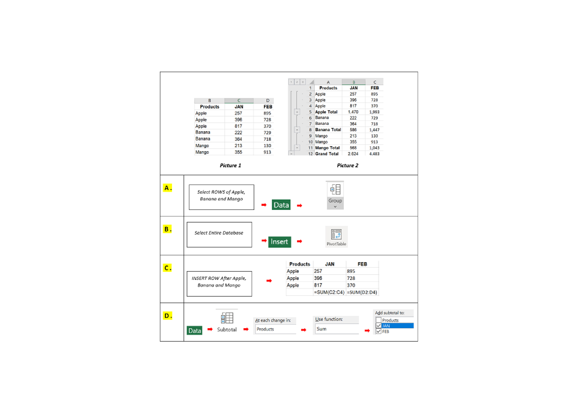
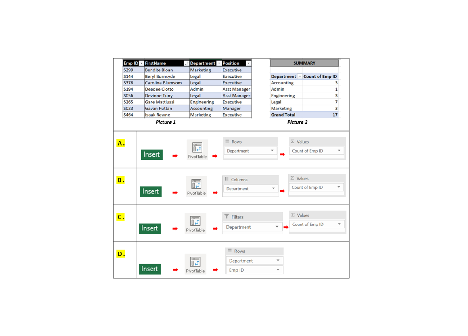
Q27. Picture 1 shows collected data. You want to summarize the data as Picture 2. Which of the following answers will allow you to achieve the result as Picture 2?
- A. SELECT ROWS of APPLE, BANANA and MANGO –> DATA (RIBBON) –> GROUP
- B. SELECT ENTIRE DATABASE –> INSERT (RIBBON) PIVOT TABLE
- C. INSERT ROW AFTER APPLE, BANANA and MANGO –> AUTOSUM FOR JAN and FEB COLUMNS
- D. DATA (RIBBON) –> SUBTOTAL –> AT EACH CHANGE IN (PRODUCT) –> USE FUNCTION (SUM) –> ADD SUBTOTAL JAN, FEB
- E. I DON'T KNOW THE CORRECT ANSWER
Question 28 of 40

28. Question
Q28. If you place non-numerical data in the Values area of a Pivot Table. What will be the result of the summary in the value area?
- A. INSERT (RIBBON) –> PIVOTTABLE –> ROWS AREA (DEPARTMENT) AND VALUE AREA (EMP ID)
- B. INSERT (RIBBON) –> PIVOTTABLE –> COLUMNS AREA (DEPARTMENT) AND VALUE AREA (EMP ID)
- C. INSERT (RIBBON) –> PIVOTTABLE –> FILTERS AREA (DEPARTMENT) AND VALUE AREA (EMP ID)
- D. INSERT (RIBBON) –> PIVOTTABLE –> ROWS AREA (DEPARTMENT) AND (EMP ID)
- E. I DON'T KNOW THE CORRECT ANSWER
Question 29 of 40

29. Question
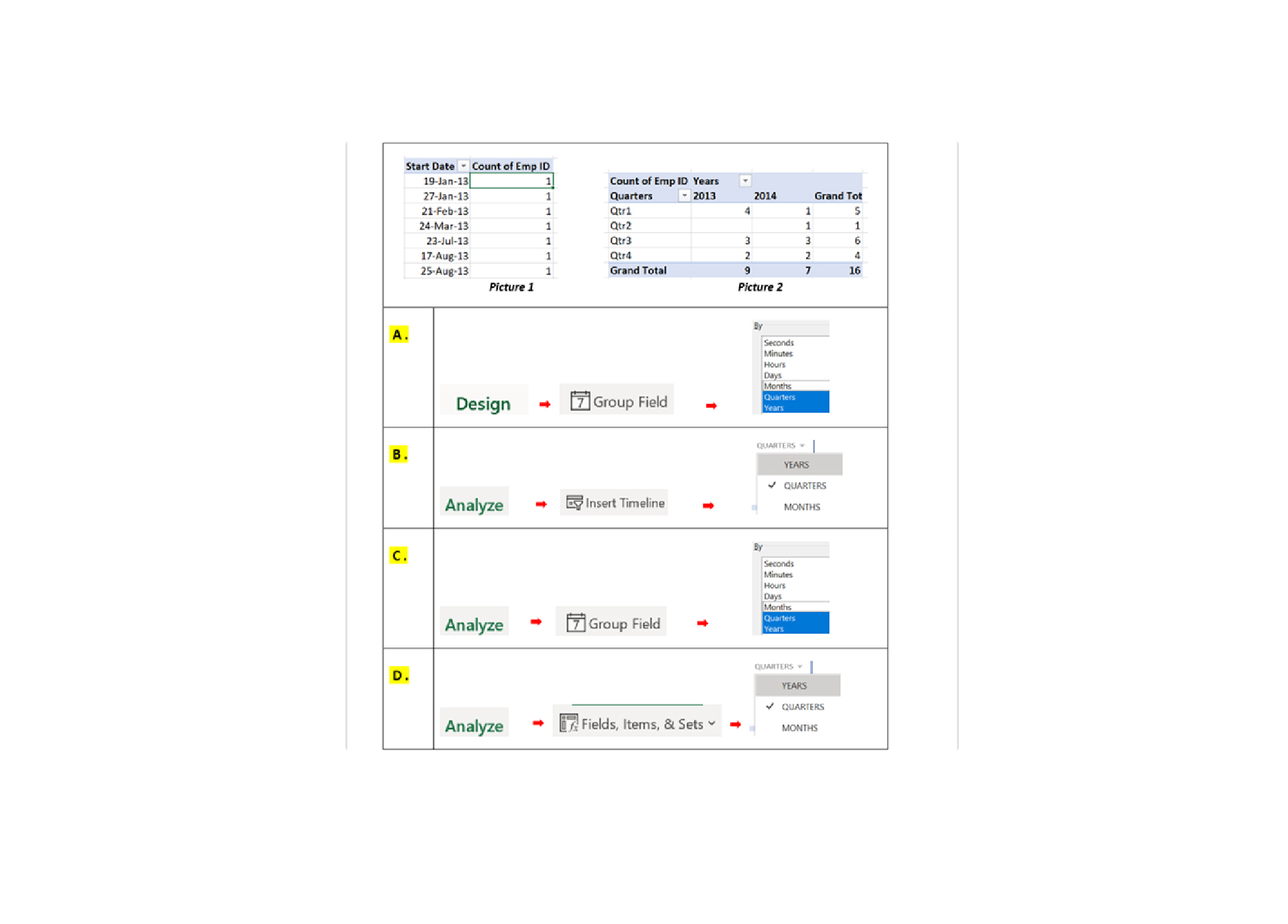
Q29. Which of these answers below is the best method to convert DAILY data as Picture 1 into QUARTERLY AND YEARLY data as Picture 2?
- A. DESIGN (RIBBON) –> GROUP FIELD –> BY (Choose QUARTERS and YEARS)
- B. ANALYZE (RIBBON) –> INSERT TIMELINE –> Choose QUARTERS and YEARS
- C. ANALYZE (RIBBON) –> GROUP FIELD –> BY (Choose QUARTERS and YEARS)
- D. ANALYZE (RIBBON) –> FIELDS, ITEMS, & SETS –> Choose QUARTERS and YEARS
- E. I DON'T KNOW THE CORRECT ANSWER
Question 30 of 40

30. Question
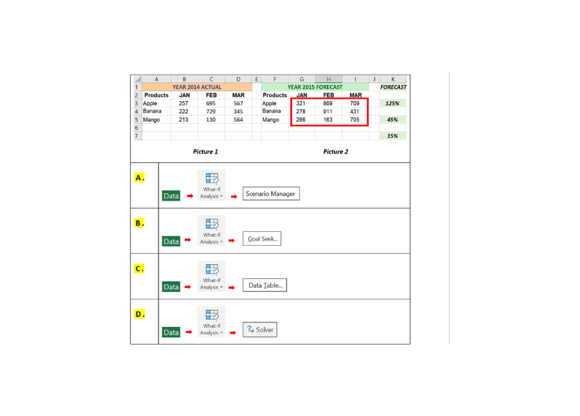
Q30. In the Sales Forecast worksheet below, you would like to show 3 different forecast values on a single spreadsheet. Which of the following answers will allow you to do this?
- A. DATA (RIBBON) –> WHAT IF ANLAYSIS –> SCENARIO MANAGER
- B. DATA (RIBBON) –> WHAT IF ANLAYSIS –> GOAL SEEK
- C. DATA (RIBBON) –> WHAT IF ANLAYSIS –> DATA TABLE
- D. DATA (RIBBON) –> WHAT IF ANLAYSIS –> SOLVER
- E. I DON'T KNOW THE CORRECT ANSWER
Question 31 of 40

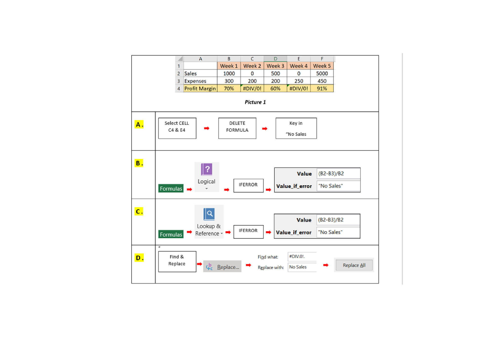
31. Question
Q31. As you can see, cell C4 & E4 show #DIV.0!. How do you prevent this in the formula?
- A. SELECT CELL C4 & E4 –> DELETE FORMULA –> KEY IN “NO SALES”
- B. FORMULAS (RIBBON) –> LOGICAL –> IFERROR > VALUE (B2-B3)/B2 AND VALUE IF ERROR “NO SALES”
- C. FORMULAS (RIBBON) –> LOOKUP & REFERENCE –> IFERROR –> VALUE (B2-B3)/B2 AND VALUE IF ERROR “NO SALES"
- D. FIND & REPLACE –> REPLACE –> FIND WHAT (#DIV.0!) AND REPLACE WITH (NO SALES)
- E. I DON'T KNOW THE CORRECT ANSWER
Question 32 of 40

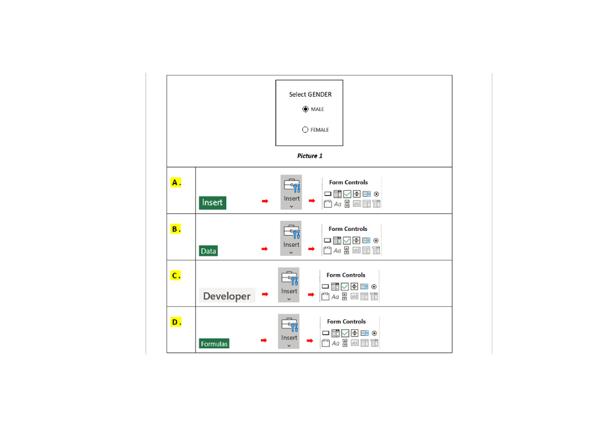
32. Question
Q32. You would like to create forms in Excel as shown in Picture 1. How do you add the Form Controls command?
- A. INSERT (RIBBON) –> INSERT –> FORM CONTROLS
- B. DATA (RIBBON) –> INSERT –> FORM CONTROLS
- C. DEVELOPER (RIBBON) –> INSERT –> FORM CONTROLS
- D. FORMULAS (RIBBON) –> INSERT –> FORM CONTROLS
- E. I DON'T KNOW THE CORRECT ANSWER
Question 33 of 40

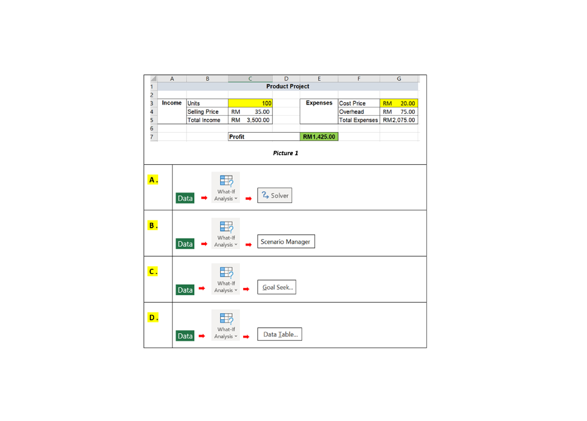
33. Question
Q33. Picture 1 shows calculation for TOTAL INCOME, TOTAL EXPENSES, PROFIT. You want to achieve PROFIT RM 10,000 by changing UNITS AND COST PRICE. How to quickly do this?
- A. DATA (RIBBON) –> WHAT IF ANALYSIS –> SOLVER
- B. DATA (RIBBON) –> WHAT IF ANALYSIS –> SCENARIO MANAGER
- C. DATA (RIBBON) –> WHAT IF ANALYSIS –> GOAL SEEK
- D. DATA (RIBBON) –> WHAT IF ANALYSIS –> DATA TABLE
- E. I DON'T KNOW THE CORRECT ANSWER
Question 34 of 40

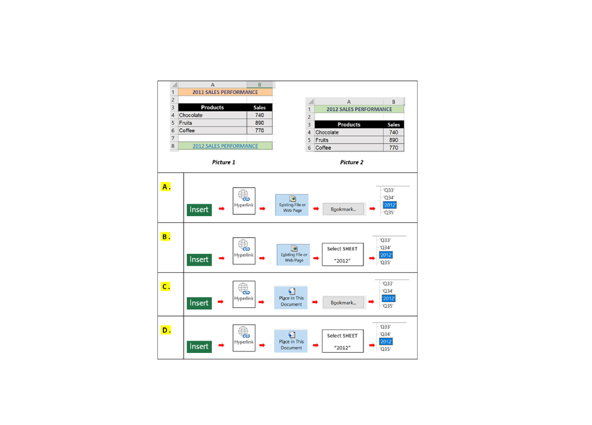
34. Question
Q34. When you click on cell A8 (Picture), it will bring you to the worksheet contains 2012 SALES PERFORMANCE as Picture 2. How do you do this?
- A. SELECT CELL A8 –> INSERT –> HYPERLINK (Existing File or Web Page) –> BOOKMARK –> 2012
- B. SELECT CELL A8 –> INSERT–> HYPERLINK (Existing File or Web Page) –> SELECT SHEET "2012" –> 2012
- C. SELECT CELL A8 > INSERT –> HYPERLINK (Place in This Document) –> BOOKMARK –> 2012
- D. SELECT CELL A8 > INSERT > HYPERLINK (Place in This Document) –> SELECT SHEET "2012" –> 2012
- E. I DON'T KNOW THE CORRECT ANSWER
Question 35 of 40

35. Question
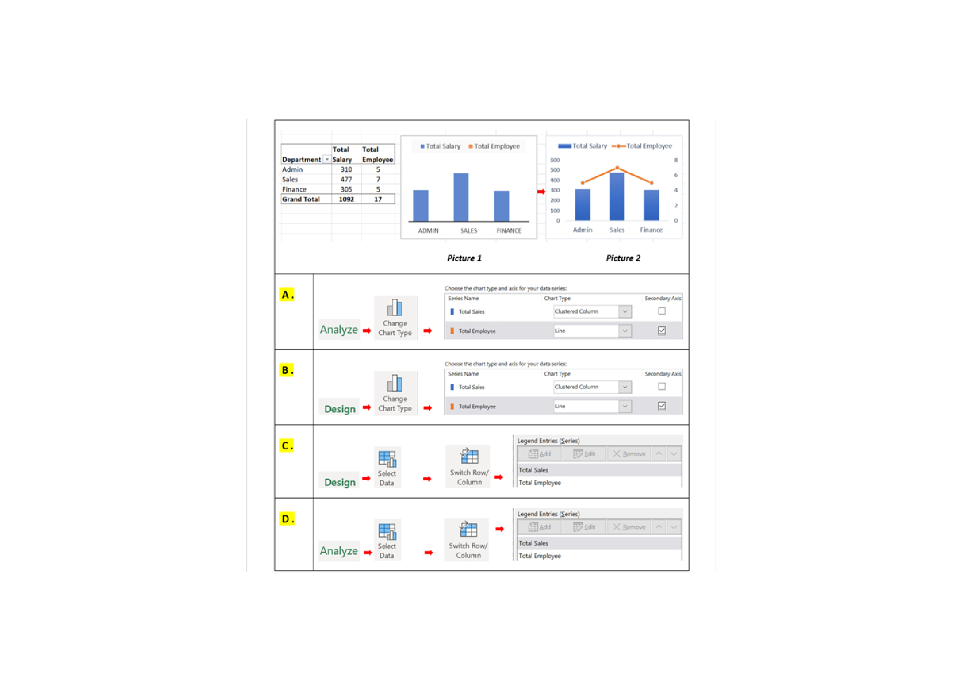
Q35. You have created a pivot chart as Picture 1. You noticed that the values for Total Employees series is not visible. How do you make visible as Picture 2?
- A. ANALYZE (RIBBON) –> CHANGE CHART TYPE –> TOTAL SALES as CLUSTERED COLUMN and TOTAL EMPLOYEE as LINE WITH SECONDARY AXIS
- B. DESIGN (RIBBON) –> CHANGE CHART TYPE –> TOTAL SALES as CLUSTERED COLUMN and TOTAL EMPLOYEE as LINE WITH SECONDARY AXIS
- C. DESIGN (RIBBON) –> SELECT DATA –> SWITCH ROW/COLUMN –> LEGEND ENTRIES –> TOTAL SALES and TOTAL EMPLOYEE
- D. ANALYZE (RIBBON) –> SELECT DATA –> SWITCH ROW/COLUMN –> LEGEND ENTRIES –> TOTAL SALES and TOTAL EMPLOYEE
- E. I DON'T KNOW THE CORRECT ANSWER
Question 36 of 40

36. Question
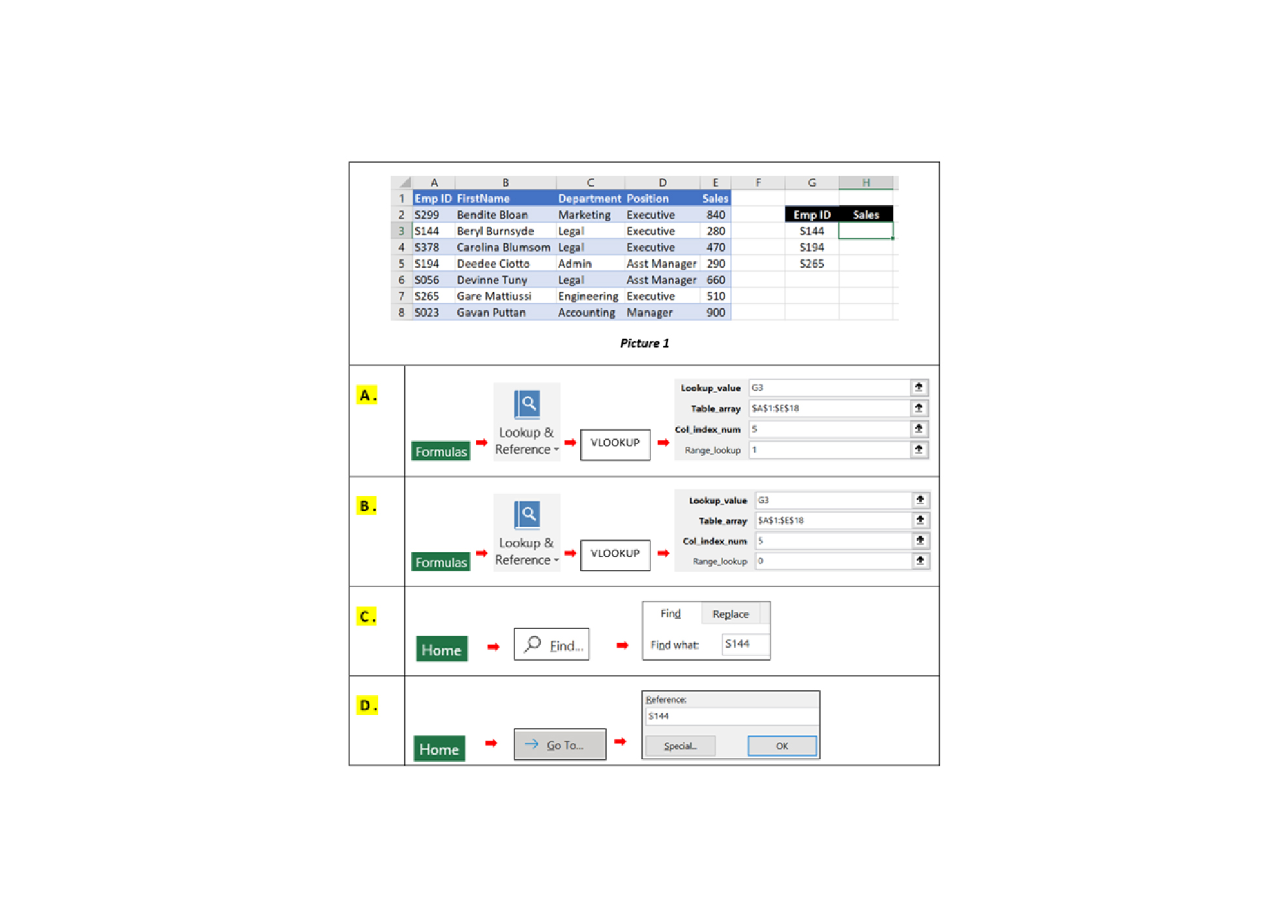
Q36. You would like to extract the Sales Value ONLY FOR SELECTED EMPLOYEE from the Sales Database. Which is the best method to do this?
- A. FORMULAS (RIBBON) –> LOOKUP & REFERENCE –> VLOOKUP(G3,A1:E18,5,1)
- B. FORMULAS (RIBBON) –> LOOKUP & REFERENCE –> VLOOKUP(G3,A1:E18,5,0)
- C. HOME (RIBBON) –> FIND –> FIND WHAT (S144)
- D. HOME (RIBBON) –> GO TO –> REFERENCE (S144)
- E. I DON'T KNOW THE CORRECT ANSWER
Question 37 of 40

37. Question
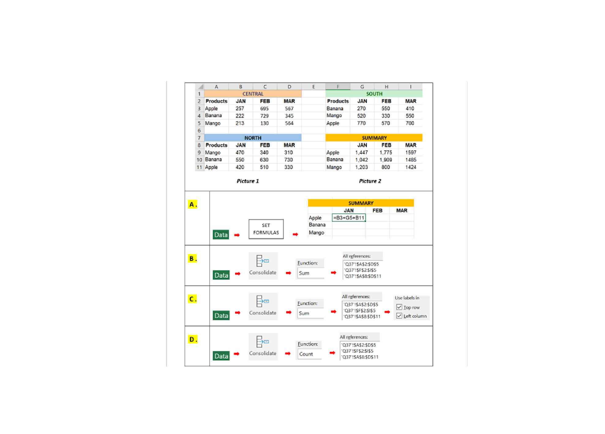
Q37. In the illustration below shows the Expenses budget for Central, North and South region. How do you summarize the values from all region into the Summary?
- A. DATA (RIBBON) –> SET FORMULAS –> B3+G5+B11
- B. DATA (RIBBON) –> CONSOLIDATE –> SUM (As Function) –> ALL REFERENCES
- C. DATA (RIBBON) –> CONSOLIDATE –> SUM (As Function) –> ALL REFERENCES –> USE LABELS –> TOP ROW and LEFT COLUMN
- D. DATA (RIBBON) –> CONSOLIDATE –> COUNT (As Function) > ALL REFERENCES
- E. I DON'T KNOW THE CORRECT ANSWER
Question 38 of 40

38. Question
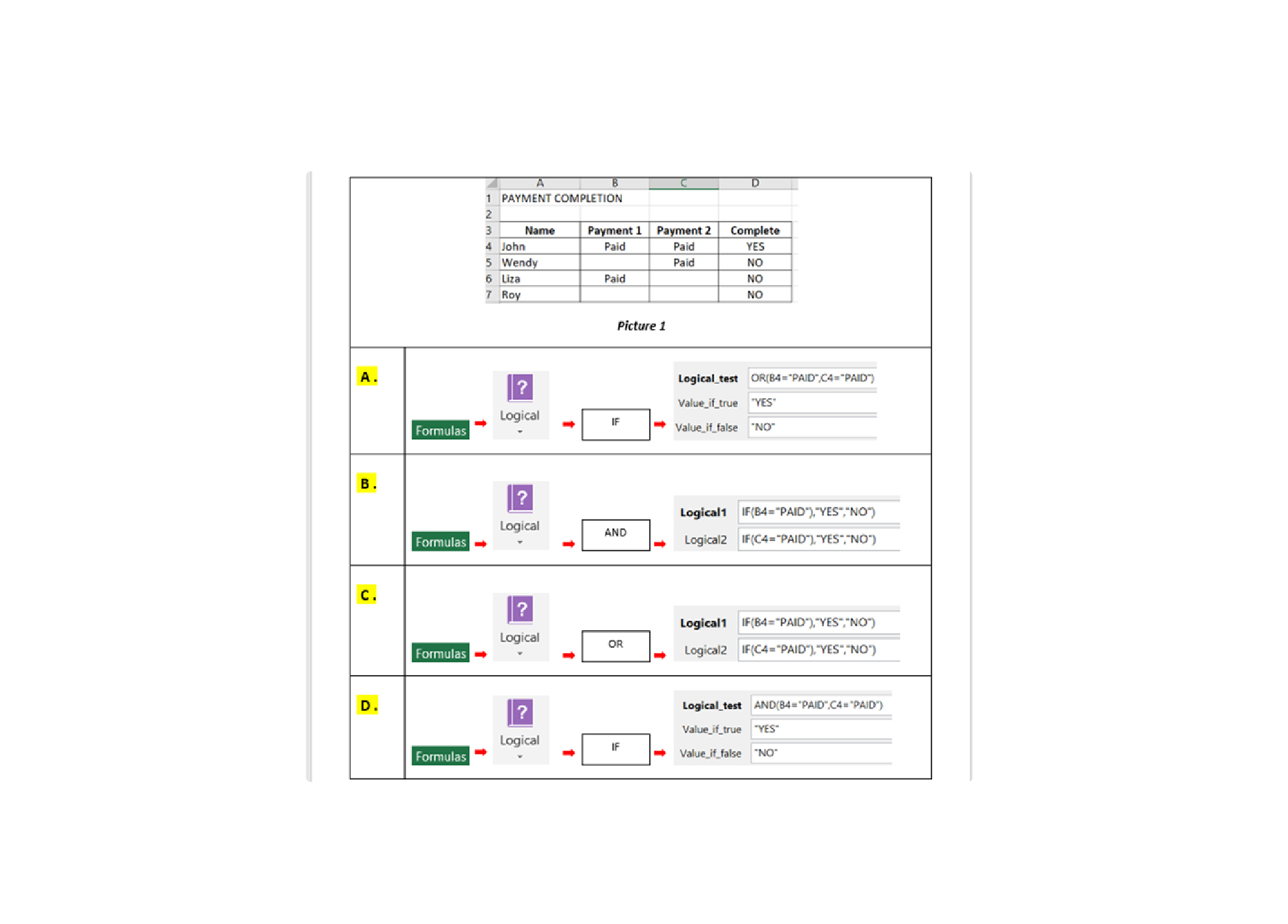
Q38. In the Payment Completion report, you would like to show the payment completion status in column “D”, as per Picture 1. Which of these answers will allow you to complete the report?
- A. FORMULAS (RIBBON) –> LOGICAL –> IF then OR
- B. FORMULAS (RIBBON) –> LOGICAL –> AND then IF
- C. FORMULAS (RIBBON) –> LOGICAL –> OR then IF
- D. FORMULAS (RIBBON) –> LOGICAL –> IF then AND
- E. I DON'T KNOW THE CORRECT ANSWER
Question 39 of 40

39. Question
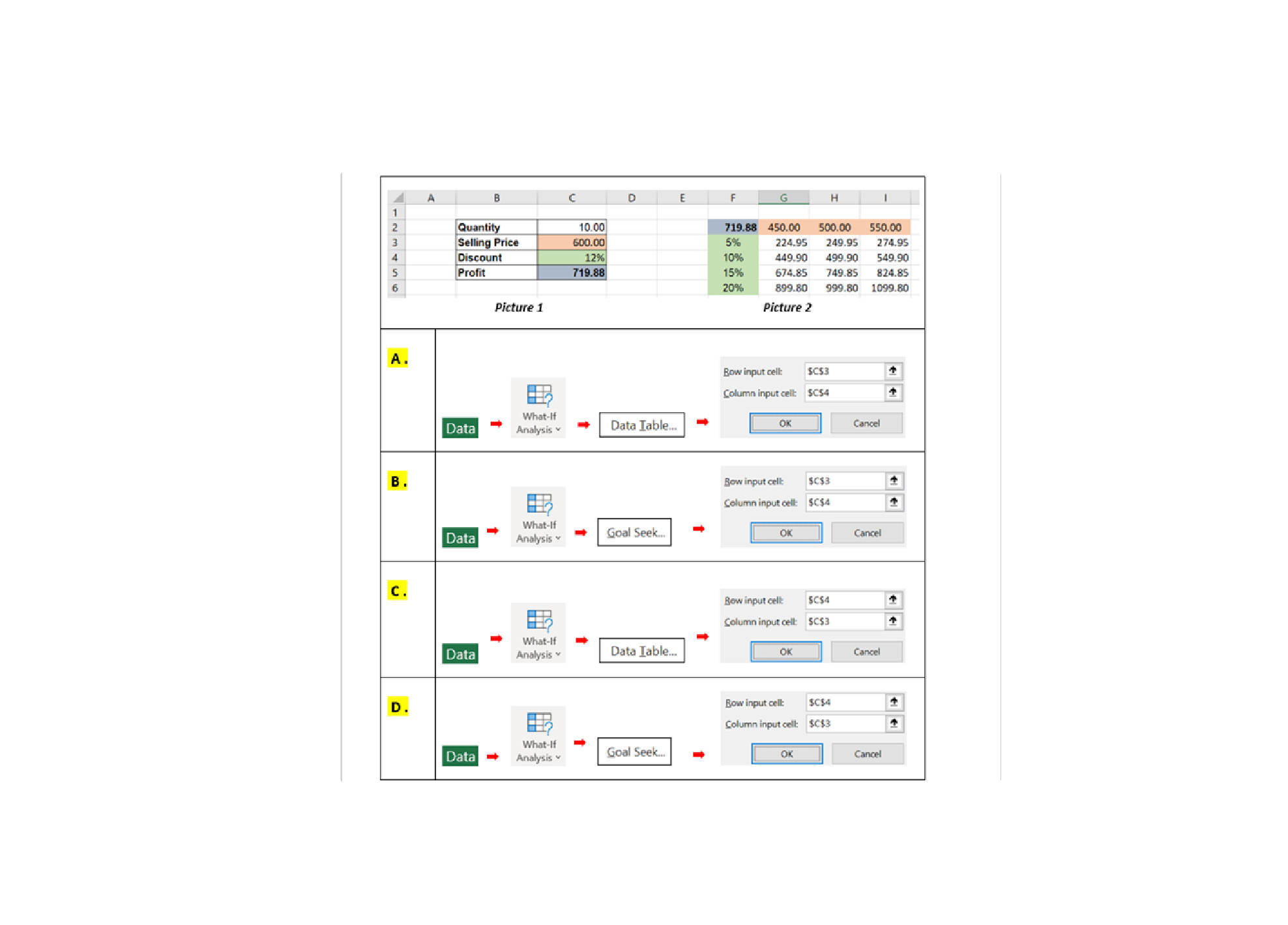
Q39. In the table as Picture 1, shows profit calculation based on Quantity, Selling Price and Discount. How do you create the table as shown in the Picture 2 to reflect profits of different selling prices and discounts?
- A. DATA (RIBBON) –> WHAT IF ANALISIS –> DATA TABLE –> C3 (AS ROW INPUT CELL) and C4 (AS COLUMN INPUT CELL)
- B. DATA (RIBBON) –> WHAT IF ANALISIS –> GOAL SEEK > C3 (AS ROW INPUT CELL) and C4 (AS COLUMN INPUT CELL)
- C. DATA (RIBBON) –> WHAT IF ANALISIS –> DATA TABLE –> C4 (AS ROW INPUT CELL) and C3 (AS COLUMN INPUT CELL)
- D. DATA (RIBBON) –> WHAT IF ANALISIS –> GOAL SEEK –> C4 (AS ROW INPUT CELL) and C3 (AS COLUMN INPUT CELL)
- E. I DON'T KNOW THE CORRECT ANSWER
Question 40 of 40

40. Question
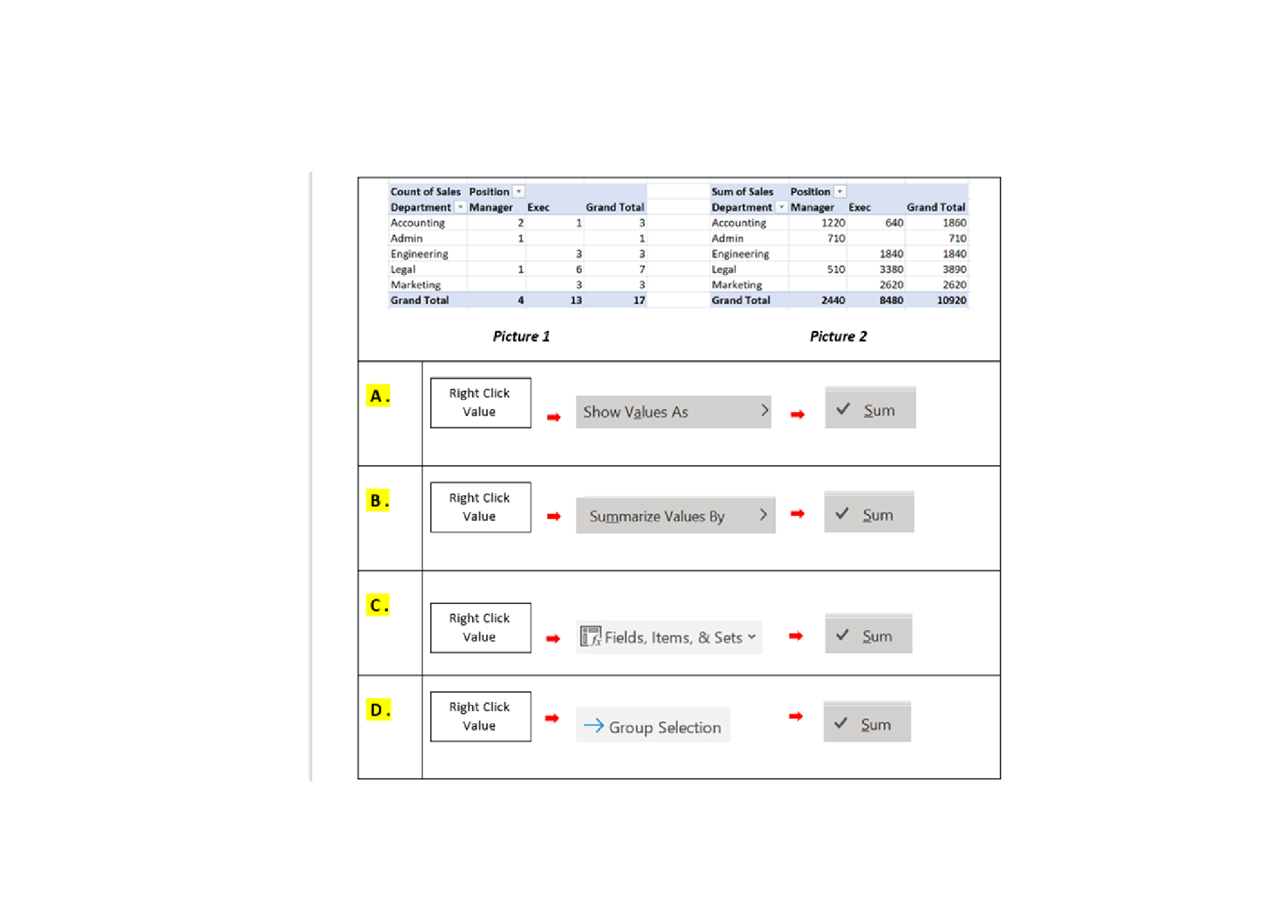
Q40. How do you change COUNT of SALES in Picture 1 to SUM of SALES as Picture 2 ?
- A. RIGHT CLICK VALUE –> SHOW VALUES AS –> SUM
- B. RIGHT CLICK VALUE –> SUMMARIZE VALUES BY –> SUM
- C. RIGHT CLICK VALUE –> FIELD, ITEMS & SETS –> SUM
- D. RIGHT CLICK VALUE –> GROUP SELECTION –> SUM
- E. I DON'T KNOW THE CORRECT ANSWER

About

Built for continuous growth, inspired by lifelong learning.
LearnLoop is a post-training learning hub automated by Edumation, designed exclusively for learners of Info Trek and Quorse.
It provides a space for participants to revise, refresh, and relearn what they’ve explored during training.

Our goal is simple: to help every learner turn training into lasting transformation through engaging, bite-sized content and continuous learning support.

Practice
Ask a Trainer

Watch & Learn
Practice
- Check My Competency
- Check My Exam Readiness
Ask a Trainer
Login

Login

Accessing this course requires a login. Please enter your credentials below!

Username or Email Address

Password

Remember Me

Lost Your Password?

Assessment Summary

Information

Results

Results

Categories

1. Question

2. Question

3. Question

4. Question

5. Question

6. Question

7. Question

8. Question

9. Question

10. Question

11. Question

12. Question

13. Question

14. Question

15. Question

16. Question

17. Question

18. Question

19. Question

20. Question

21. Question

22. Question

23. Question

24. Question

25. Question

26. Question

27. Question

28. Question

29. Question

30. Question

31. Question

32. Question

33. Question

34. Question

35. Question

36. Question

37. Question

38. Question

39. Question

40. Question

About